A good Yet-to-Find analysis starts with a good map. Photo of a geological map of Pakistan compiled by BPM, 1956. Photo: Henk Kombrink
Why USGS Yet-to-Find figures are an overestimation
A commercial decision to make a move into a basin is something you need Yet-to-Find (YTF) volumes for. But how do you arrive at a reasonable estimate of YTF?

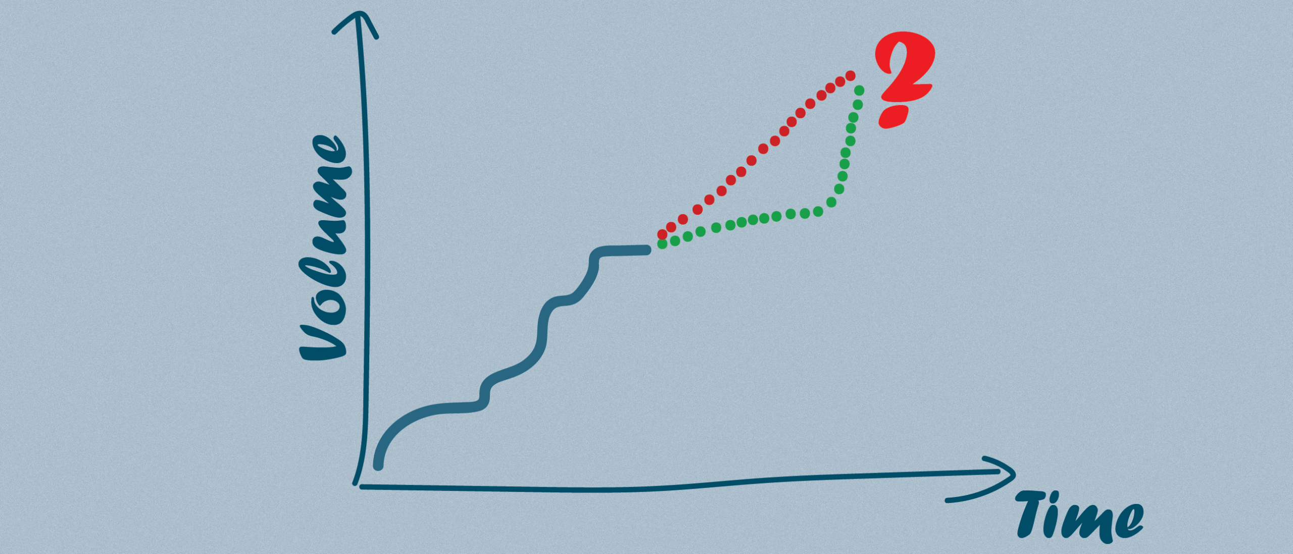
One of the most common ways to estimate YTF is the extrapolation of discovery rates, as can be calculated from a creaming curve. However, this methodology does not have any guidance on discovery size – is it just a single big one or lots of smaller pools? “Hence, we think it is not a very useful tool. Because what we really try to find are the large fields that are still out there, even in mature basins,” says Ian Longley from GIS-Pax in a recent video.
Then there is basin modelling. “However,” says Ian, “I always think about the following infamous and inaccurate quote from Jad Babbin, former US Secretary of Defence: “Going to war without the French is like going deer hunting without an accordion. You just leave a lot of useless, noisy baggage behind”. I feel the same way about the role of basin modelling when it comes to predicting a YTF estimate, because of the sheer amount of uncertainty in most of the inputs, especially hydrocarbon migration losses and the uncertainty it brings.”
The most famous methodology is the one championed by ExxonMobil: Play maps with predicted prospects. Without going into much detail, it captures the main elements of each play in a map framework, which is followed by the integration of these elements into basin-wide maps. This can be quite an extensive process, and not all companies have the resources to do this. But there is a shortcut.

“Rather than looking at the entirety of a basin or a country, what we suggest is to only focus on the proven charge areas, where we know hydrocarbons have been generated and success rates can be calibrated,” explains Ian. “That way, we eliminate large areas where a detailed analysis would always be speculative at best. Within these proven charge areas, we only produce one risk map, which is calibrated by the local exploration results. When combining this with a prospect inventory, which we have access to through a collaboration with S&P Global, we can subsequently provide a global exploration risk map that we then split up in 19 different stratigraphic intervals or plays.”
The best way to then find the Yet-to-Find estimates is to identify each mapped prospect and aggregate the mean risked volumes to arrive at a YTF estimate. “As a final step, we also introduce a methodology to estimate how many unknown prospects there still are out there, following the methodology outlined by Hood et. al. (2023).”
Why is this workflow better than the one applied by the USGS? “Because they apply the same exploration risk across entire area basin polygons and do not use real prospects, where we rely much more on sub-areas where the proven source areas are our main focus areas,” says Ian. “As a result, the USGS YTFs tend to be approximately three times as high as ours. In turn, this has a serious implication on how much oil there is still out there to be found. We won’t claim that our technique is without its assumptions, but we do believe that it is more accurate than the UGGS’s estimate at least.”
This is the ninth of a series of articles based on work and experience from the GIS-Pax team in Australia, as presented by Ian Longley in a series of videos on LinkedIn.
Find the previous articles here:
Why the Term “Fault Block” Is a Useless Way to Describe a Trap
Why Traffic Light Play Maps Are Useless
Why Peer Reviews Often Don’t Work
Why P10/P90 Prospect Ratios Are Meaningless Without Involving the Geology
Understanding the “Minimum Economic Field Size” concept and aggregating targets
Why post well analysis matters
Why amplitude-supported prospects are not the silver bullet we are led to believe