A Simple Guide to Seismic Amplitudes and Detuning
Seismic Amplitudes
 Data processing such as detuning reveals the true sweetspots in your data.In a seismic survey, seismic amplitude is a measure of the contrast in properties between two layers. If the data are converted to relative impedance then seismic data observe the relative change of the rock property impedance (= hardness) as we move from one layer to the next. Note that seismic cannot tell us about the absolute change, only about relative changes.
The rock property contrast between a sand and shale varies with factors such as depth of burial, compaction, porosity and lithological composition. The amplitude response could be positive, negative or negligible depending on the relative hardness of the sands to the encasing shales. If we have an extensive reservoir sand, perhaps a sheet flood, beneath a shale, then the amplitude might vary laterally due to porosity variation or changes in reservoir quality by as much as 10–20% and these amplitude changes may be interpretable in terms of property changes. In a soft sand, the presence of gas will lower the impedance significantly, making a negative amplitude even more negative and therefore brighter (Figure 1). We can consider this in terms of reflection amplitude (for conventional seismic data) or relative impedance (for inverted data; see ‘A Simple Guide to Seismic Inversion’). Amplitude effects can be interpreted more easily on relative impedance data as the inversion process converts the reflection contrast to a local rock property.
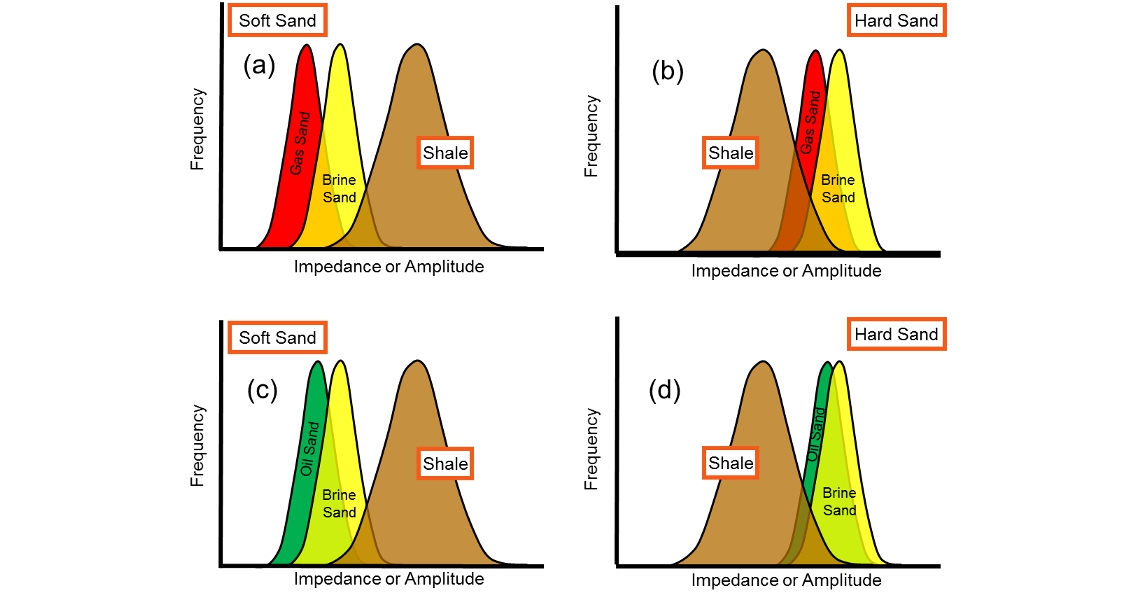
Figure 1: Representative histograms of seismic impedance for hard and soft sands with brine, oil or gas. Left: sands softer than shales; right: sands harder than shales. (a) gas sand has larger separation to low impedance than oil sand in (c). In hard sands, hydrocarbon effects move the response towards shale properties in (b) while gas sand shifts to lower impedance but starts to overlap shale properties. In (d), an oil sand produces a less pronounced change than would be seen in a soft sand.
For a picked horizon, if we extract amplitudes and present them as a map, the pattern of amplitudes may tell us something about the geology. In order of magnitude from strongest to weakest, physical property changes that might result in amplitude effects that we might see and interpret on seismic are typically lithology, porosity, gas fluids and oil fluids.
A common application of amplitude maps is to compare amplitudes to structure, as conformance of an amplitude anomaly with structure may indicate a direct hydrocarbon indicator, or DHI. This is usually assessed visually.
Saturation and pressure (time lapse effects) due to production may also be observed in seismic. These effects are much smaller and require repeat seismic surveys to be acquired and compared to each other over time, hence timelapse surveys.
Tuning Effects
The earth is comprised of many geological layers superimposed on each other. Seismic data records only a limited range of frequencies (bandwidth), typically 10–60 Hz. (In terms of music, you feel rather than hear sounds at the lowest of these frequencies, the lowest note on a 4-string bass guitar being about 41 Hz). Consider a single layer: as it thins, the seismic reflection from the top and the bottom of the layer get closer together until eventually they begin to overlap, which results in interference. If we compute the relevant impedance for, say, a blocky sand, where the sand properties are fixed and only the thickness changes, we find that the seismic amplitude varies significantly with the thickness. As the layer thins, the amplitude brightens due to constructive interference, reaches a peak and then declines due to destructive interference when the layer becomes very thin. This brightening due to constructive interference is thickness dependent tuning – usually just called tuning.
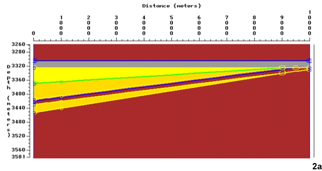
Figure 2a: Example of a tuning wedge model. The thinning sand wedge model is shown in 2a. The internal properties of this layer model are constant, only the thickness changes, forming the wedge. (Modified from Francis & Syed, 2001)
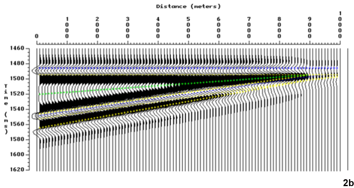
Figure 2b: Conventional seismic reflection response of this wedge model. Note how the black events merge together as the wedge thins to the right. (Modified from Francis & Syed, 2001)
Geophysicists show the effect of tuning using a constant property wedge model. An example of this type of model of a thinning reservoir is shown in Figure 2 (above and below). Image 2a is the wedge model for brine saturated sand, where all the layers in the model have constant properties: only the thicknesses are changing, thinning from left to right. In Figure 2b we see what this model would look like as seismic reflection data, where the black events merge into a single event on the righthand side. Figure 2c shows the resultant relative impedance, where the reservoir interval appears as the yellow and green coloured (low impedance) layers. The actual modelled interval (2a) has constant impedance within each layer, but the relative impedance from the seismic model response is clearly brighter (greener) in the centre and reduces in amplitude (yellower) as the interval gets thicker or thinner.
Figure 2d shows a plot of amplitude (from the yellowgreen sand in 2c) versus time thickness of the wedge. Note how the amplitude reaches a maximum around 13 ms and then falls off to about half the peak amplitude at around 35 ms. This doubling of the amplitude as a function of thickness is the tuning effect.
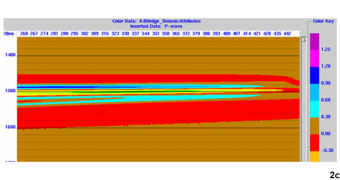
Figure 2c: Relative impedance amplitude response derived from the seismic response in (b). The sand wedge shows as the yellow-green colours. Note the brightening to strong green in the centre of the wedge model – this is the tuning effect caused by the thickness change. (Modified from Francis & Syed, 2001)
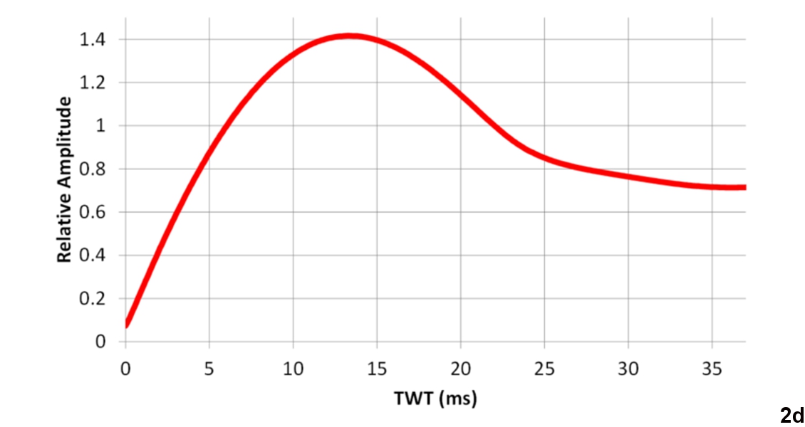
Figure 2d: Plot of the amplitude from (c) against the thickness of the sand in time. (Modified from Francis & Syed, 2001)
Modelling of the effect of gas in the same field demonstrated that a gas-filled reservoir sand would have about a 25% brighter amplitude than a brinefilled sand. From Figure 2d, the effect of changing reservoir thickness from 36 to 13 ms (corresponding to a thickness change from 60 to about 20m) would be to double the maximum amplitude of the seismic reflection, clearly demonstrating that thickness-related tuning effects are potentially much larger than lateral amplitude variations due to geological changes, including lithology or hydrocarbon fluid effects.
Tuning Effects and Amplitude Maps
Tuning effects are very predominant in seismic amplitude responses and tend to be the most significant factor affecting amplitude maps. Meaningful interpretation of amplitudes in terms of lateral property changes therefore requires us to first remove the effects of tuning.
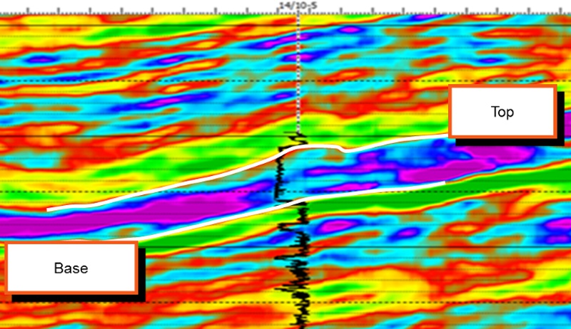 Figure 3: Picking top and base zero crossings to define the thickness and amplitude of a hard sand from relative impedance seismic inversion data.To extract amplitude maps from seismic data we need a consistent approach. Fortunately, if we interpret on relative impedance data, there is a natural choice of how to pick and extract amplitudes – by picking zero crossings (Figure 3).
To correct amplitude maps for tuning, we need to first define the tuning curve as in Figure 2d, either by modelling or empirically from seismic picks (as discussed below). On the tuning curve, we arbitrarily define a reference for the seismic response. This is often convenient if set to be about half the peak tuning amplitude, or 0.7 in the example in Figure 2d. If our target interval had no property variation we would expect the seismic amplitude to be constant at all thicknesses if we remove the effect of tuning. So at any thickness we multiply the seismic amplitude by a factor which is the ratio of the reference amplitude to the tuning curve value at that thickness to correct the value on the orange curve to the reference value. As this is just a ratio, the scaling is arbitrary; if we know the shape of the tuning curve as a function of thickness we can detune amplitude data.
Figure 4 shows an example of amplitude detuning of a hard sand turbidite. The picked time thickness for the fan is shown in Figure 4a and the corresponding amplitude map in 4b. Note the bright amplitudes in the distal (south-west) end of the fan, associated with thinner intervals in the time thickness map; these are the result of tuning. Using the thickness and tuning curve information, detuning results in the amplitude map, 4c, where, after detuning, the prominent bright features are relatively suppressed and larger areas of the fan now show similar amplitudes.
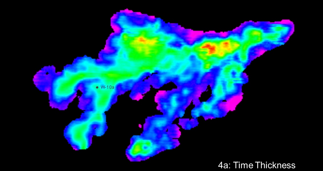
Figure 4a: Time thickness map for a turbidite fan picked on top and base zero crossings from 3 D seismic.
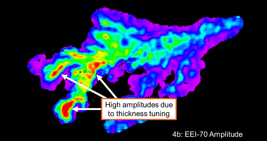
Figure 4b: Average amplitude map between the top and base zero crossing picks from (a). Note that the bright amplitudes in the distal (southwest) area of the fan are associated with thinner intervals in the time thickness map. These bright, high amplitudes are the result of tuning.
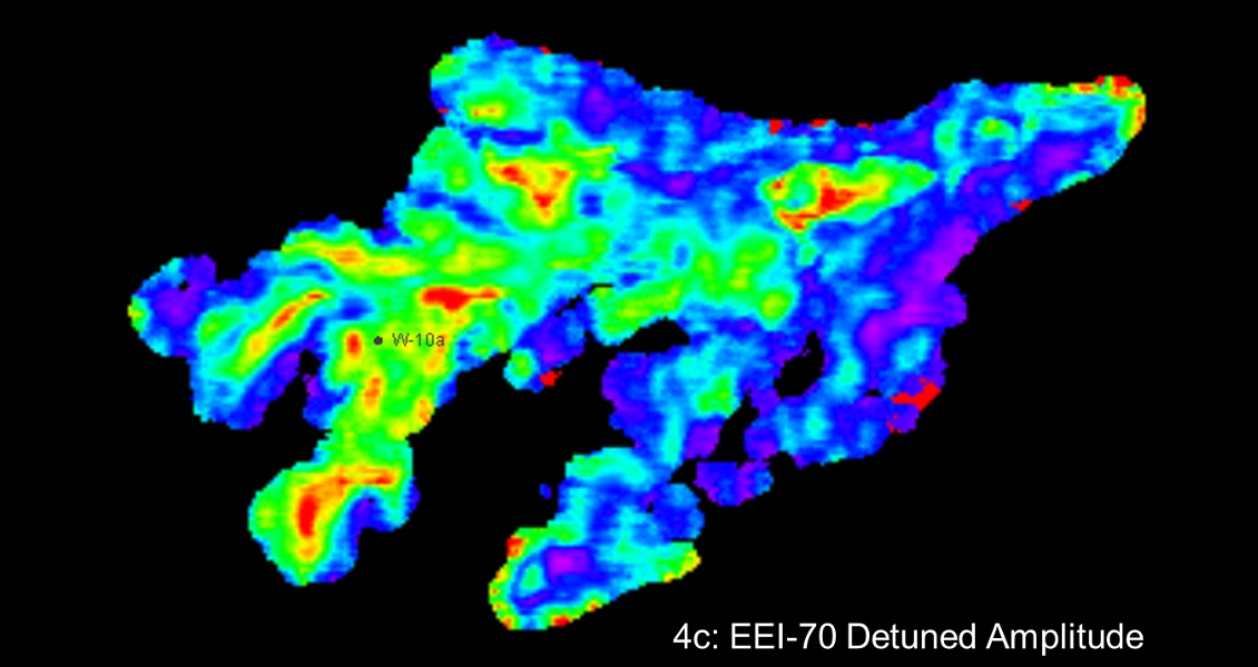
Figure 4c: Using the thickness and tuning curve information (Figure 5), results in the detuned amplitude map (c). Note how, after detuning, the prominent bright features are relatively supressed and larger areas of the fan now show similar amplitudes.
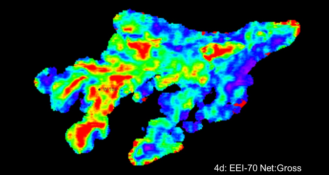
Figure 4d: Amplitude map of (c) calibrated to N:G using the method of Connolly (2007).
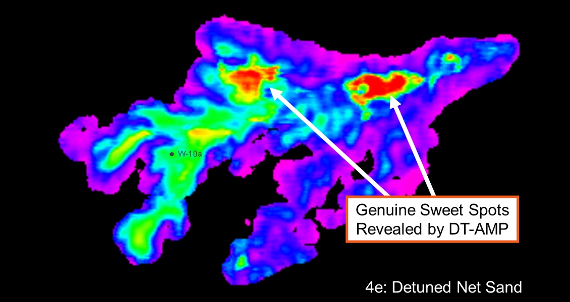
Figure 4e: Net sand map, obtained by multiplying the net:gross quality of (d) by the time thicknes of (a) and also multiplying by the sand velocity to obtain a net reservoir thickness estimate in metres, again using the method of Connolly.
Tuning Curves and Net Sand
Having interpreted the top and base zero crossings for the selected seismic event, we can cross-plot the average amplitude versus TWT interval thickness for every interpreted trace. Using the data from Figure 4a and 4b, an example of a tuning curve crossplot is shown in Figure 5. The orange line shows the expected amplitude versus TWT thickness relationship for a clean sand – this curve was used for detuning the data and obtaining the result in Figure 4c.
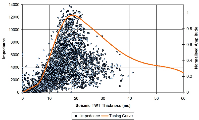 Figure 5: Crossplot of average amplitude against time thickness with modelled tuning curve superimposed.Inspection of Figure 5 shows that for real data sets there is a cloud of points rather than a simple curve relating amplitude to thickness. For every thickness there is a wide range of observed amplitudes. Why is this?
In 2007 Pat Connolly published a paper in The Leading Edge describing how the spread of amplitudes at a given thickness can be related to a change in reservoir properties, notably reservoir quality or net:gross (N:G). The argument is that if the ‘reservoir’ interval had the same properties as a shale above or below, then there would be no amplitude because there would be no contrast. An amplitude close to zero would be 0% N:G and would plot at the bottom edge of the graph. At the top of the graph, the orange curve represents the sand line where the N:G would be 100%. The position of any sample vertically can then be interpreted in terms of reservoir quality, so a point at half amplitude would be 50% N:G. For a given time thickness, the ratio of the observed amplitude to the tuning curve (100% sand) is then both a rock quality measure (N:G) and, because it also takes into account the shape of the tuning curve, is also detuned (Figure 4d). Figure 4e shows a net sand map, obtained by multiplying the N:G map of 4d by the time thickness of 4a and also multiplying by the sand velocity to obtain a net reservoir thickness estimate in metres.
3D Seismic Detuning
So far detuning has been described here in terms of corrections applied to 2D maps, but it would have far more application if it could be applied to 3D seismic. In A Simple Guide to Seismic Inversion it was noted that seismic inversion output is potentially attractive as a constraint in reservoir modelling, but the effects of tuning must be removed from a relative (coloured) or deterministic inversion before use, so it would be of great value if a 3D reservoir model included detuned 3D seismic data.
Figure 6a shows a seismic section through a coloured impedance volume for the hard sands. At the well in the centre of the section the sand is close to 100% N:G. Bright amplitudes are developing downdip to the left, sustained all the way to the second well, and the reservoir is also thinning downdip. The downdip well has a lower N:G having some shalier intervals, so why are these amplitudes brighter downdip than at the thicker sands in the well at the centre of the section? The answer is, of course, tuning!
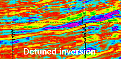
Figure 6b is the same seismic cross-section after the application of a new method of 3D seismic detuning called DT-AMP. The output is called the detuned modulated amplitude (DMAMP). After detuning, the bright amplitudes downdip are clearly removed and the change of amplitude now reflects the seismic interpretation of the rock properties: downdip there is a deterioration in reservoir quality.
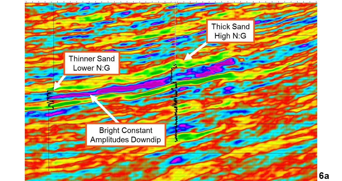
Figure 6a: Seismic relative impedance for a hard sand turbidite from the Sea Lion field. Original relative impedance seismic response, hard sands show as the strong blue/purple response. Note brightness downdip from the well in the centre to the well on the left.
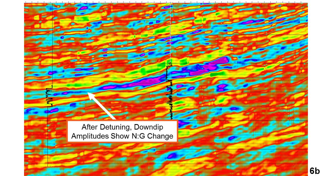
Figure 6b: Seismic relative impedance for a hard sand turbidite from the Sea Lion field. Relative impedance after 3D seismic detuning using DT-AMP to remove tuning effects. Downdip brightening due to thickness related tuning is now suppressed and the amplitude better represents the lateral change to lower N:G in the down-dip well.
In fact, I should come clean. All the amplitude and thickness displays shown here were generated by detuning the 3D seismic directly. The intermediate output products of this method allow very rapid, automated picking of the time thickness, average, detuned and N:G amplitudes. Manually picking the top/base zero crossing for the multiple fans in this survey originally took around six weeks; using 3D seismic detuning, a fan can be reliably picked and mapped in less than a day. And the 3D seismic is detuned in situ – so now where’s my reservoir model?