Benjamin and William Franklin risked their lives when conducting their famous lightning experiment in Philadelphia in 1752. A simple silk kite was sent aloft in a storm. A wire at the top served as a lightning rod. The kite was connected to a hemp string – which when wet would conduct any electrical charge from the storm down to a metal key. As the hemp line became wet, they noticed loose threads of the hemp string standing erect. Benjamin touched the key, and as the negative charges in the metal were attracted to the positive charges in his hand, he felt a spark. This experiment did not discover electricity, but it clearly demonstrated the connection between lightning and electricity.
Dynamic Measurement’s path to discovery similarly took a path less travelled. Joe Roberts accidently put his life on the line while hunting ducks on his property on the edge of the Hockley Salt Dome in southern Texas, when a lightning strike hit very close to him, terrifying him. The same thing happened a year later, in exactly the same place. He drove round to his friend Roice Nelson, geophysicist and co-founder of Landmark Graphics Corporation, and asked, “Does lightning strike twice in the same place; if it does, does it mean I have oil on my property?” Roice asked Dr. Jim Siebert, Chief Meteorologist at Fox News in Houston, the same questions. Discussions with other experienced geophysicists, including Les Denham, resulted in the formation of Dynamic Measurement LLC. All three authors have had close experiences with lightning strikes, and Joe’s experience rang true to us.
We have now conclusively demonstrated that lightning does strike the same place twice. In fact, lightning strikes cluster, and these clusters are somewhat consistent over time. Dynamic Measurement continues to discover relationships between lightning strikes and resistive natural resources like aquifers, geothermal deposits, oil & gas reserves, as well as conductive materials such as copper, gold, silver, iron, kimberlite pipes, gemstone deposits, clays, and brines. Neither repetitive strike locations nor the presence of resistive/conductive actors under them are random.
(For clarity: the entire lightning path is generally referred to as a stroke, while the location the stroke hits the ground is the strike.)
Lightning Strikes
On a clear day the earth’s surface acts as an equipotential surface, with equipotential lines parallel to the topography. Electrons cluster at a point like an antenna – or Benjamin Franklin’s kite. We are connected to the earth’s electrical circuit, and the equipotential lines go up around us or the lightning rod. The electric field lines are always perpendicular to these equipotential lines.
At the micro scale close to the earth, as static charge builds up in the atmosphere when an electric storm passes, the static electricity moves along field lines, and bleeds into the earth, including, to a miniscule degree, to derivatives of Franklin’s lightning rod. At the macro scale, ice and dust particle collisions within the clouds at 600–900m (2,000 – 30,000ft) above the earth’s surface generate electrical charges. Cloud-to-cloud (C2C) strikes result when opposite electrical charge build-ups in the clouds exceeds the dielectric, the electrical insolation of the air.
A basic assumption we make is that this build-up of charge interacts with telluric (earth) currents, at depths proportional to the height of the clouds where the charge originates.
The atmospheric electromagnetic half-space mirrors the earth’s electromagnetic half space. During the minutes or hours during which the static charge builds up in the clouds, the charge interacts with and induces telluric currents. A signal with period of 24 Hz is generally believed to have a skin depth of 600-800 km (375-800 miles).

Lightning strikes are understood to have a skin depth of a few metres. We know lightning strikes are a major source for charging telluric currents, all the way to the Mohorovičić discontinuity, at the base of the crust at a depth of 10-90 km (6-55 miles), and everything below the Moho is believed to be molten, and therefore a good conductor.
Lightning storms build up over hours, lightning strikes over milliseconds, and this build-up of static electricity in the atmosphere is what charges telluric currents, and what interacts with these currents to guide lightning strike locations.
Geophysicists have known atmospheric static currents charge telluric currents since the 1950s, with the invention of magnetotellurics as a geophysical exploration technique. The build-up to a lightning strike takes up to 500 ms and can be derived by summing the time for related Cloud-to-Cloud (C2C) and Cloud-to-Ground (C2G) strikes.
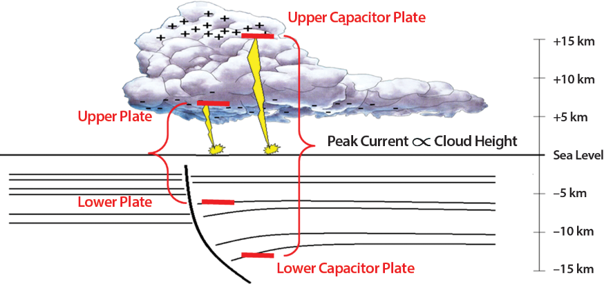
This build-up of atmospheric charge identifies an area of opposite charge in the subsurface of the earth. Lightning stroke pathways are largely determined by the field lines connecting these two ‘capacitor plates’.
Earth as Capacitor
Meteorologists have been studying atmospheric electrical currents for decades. NASA satellites provide a different viewing angle, and have provided a much clearer understanding of how electrically charged clouds interreact with the upper atmosphere. A lot is now known, but there is a lot yet to be unravelled. The atmosphere is very fluid, and it is not simple to measure electric fields and equipotential surfaces in and around clouds. The electrical conductivity of air is 0.3-0.8 x 10⁻¹⁴ Siemens per meter, considerably lower than the earth’s, which explains the effectiveness of using air to separate high voltage transmission lines from the ground using towers to support transmission lines in the air. The earth is much more conductive than air: assuming a typical sedimentary rock has 5% porosity, the electrical conductivity is 5.0 x 10⁻⁴ Siemens per meter, or about 1010 times the conductivity of air.
Treating the atmosphere and the earth as a capacitor, the charged thunder cloud can be considered one plate, while the other is the earth underlying the charged cloud. The dielectric is the insulating medium between the capacitor plates that transmits electrical force without conduction; namely the air and the earth, between the atmospheric static charge build-up and the interacting and oppositely charged currents in a different part of the thunderclouds (C2C strokes) or telluric currents at depth (C2G strokes). Dynamic makes two assumptions: firstly, lightning occurs when there is sufficient charge to bridge the capacitor; and secondly, lightning is affected by geology to a depth proportional to the cloud height, as estimated from the Peak Current of the stroke. We recognise it is hard to accurately measure the height of a lightning stroke, and that the lightning strike itself, lasting microseconds, is a small part of the electrical interaction between the atmosphere and the lithosphere.
Lightning is like a current along a wire, inducing a magnetic field, which interacts with telluric currents deep in the subsurface. These telluric currents have more impact on lightning strike locations than vegetation, infrastructure, or topography. There is extensive professional literature on magnetotellurics, ElectroSeis, Tipper and other geophysical exploration techniques based on passive measurements of lightning induced currents.
The bottom line is lightning is a meteorological event most often associated with storm clouds.
Lightning seldom occurs in the extreme northern and southern latitudes, over deep water, or in some deserts, meaning there will be less lightning data in these areas for lightning analysis.
The North American Lightning Detection Network, containing 20 years of data from the US and Canada, is the most extensive lightning database available, with records of location, time, Peak Current, Peak-to-Zero Time, recording quality, and other attributes. Most strikes in the US are recorded by 10–25 sensors, each within about 1,000 km of the strike location. These data are collected and stored for insurance, safety, and meteorological reasons, but Dynamic Measurement’s exclusive data licence for natural resource exploration highlights new uses for them.
To illustrate how lightning analysis can be used in hydrocarbon exploration, let’s look at examples from the Corpus Christi area of South Texas and from South Utah.
Lightning for Exploration – Example: South Texas
These figures to compare regional lightning analysis results with geological ground truth, using work by Tom Ewing at the Bureau of Economic Geology (BEG). Dynamic Measurement has patented a method of calculating apparent resistivity from the lightning databases as a direct calculation, not an inversion process. The mathematical model is based on a relaxation oscillator (a neon light tube), where a capacitor is in series with a resistor and in parallel with a spark gap. As an input voltage is built up on the capacitor, it creates a spark across the gap, causing the inert gas to fluoresce. With a lightning strike, there is an additional resistor between the capacitor and the spark gap: namely the apparent resistivity of the earth between the strike location and where the telluric currents form the base plate of the capacitor.
As lightning leaders come down from the clouds, opposite charged electricity at the surface collects and moves upward as a streamer of the opposite charge, and the up-going streamer and the down-going lightning stroke meet, the path is ionised and there is almost no resistance. The resistance in the subsurface is approximately constant over long periods of time, so even though each storm is unique and atmospheric factors vary with each stroke, with millions of strikes the consistent geological electrical properties result in strikes and attributes clustering.
Estimating the top capacitor ‘cloud height’ from Peak Current provides an estimate the base capacitor depth. Placing the calculated apparent resistivity (or other lightning attributes) at these depths and doing a 3D interpolation allows the creation of an apparent resistivity (or other lightning attribute) volume. These volumes can be interpolated to provide a trace for each bin in an existing or planned 3D seismic survey, or each grid point in an aeromagnetic survey. Binning, and averaging all resistivity or other lightning attribute values for a specific area, creates a map of the sum of the specific lightning attribute or rock property being evaluated.
These volumes or maps, created anywhere there is Rise- Time, Peak Current, and Peak-to-Zero lightning strike data, can fill the gap between existing seismic and geophysical control. In the case of apparent resistivity, measurements are not limited to a few inches from the well bore, as with well resistivity logs. These lightning derived attribute and rock property maps and volumes provide a cost-effective geo-framework for all geological and geophysical data and interpretations.
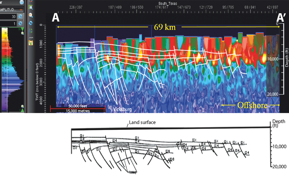
Here is a cross-section and a horizontal slice through the Stratton Field taken from about 30 km west of section A–A’ in the previous image. In this display the seismic data released by the BEG is semi-transparent, revealing the apparent resistivity underneath. A Vicksburg expansion fault (dashed green line) is easy to see on the seismic data: note how well the resistivity volume maps this fault out from the seismic control. The fault can also be seen on the 2,000 ms time-slice on the right.
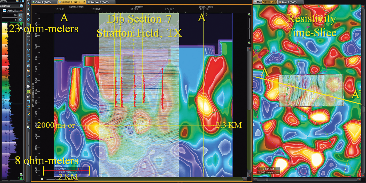
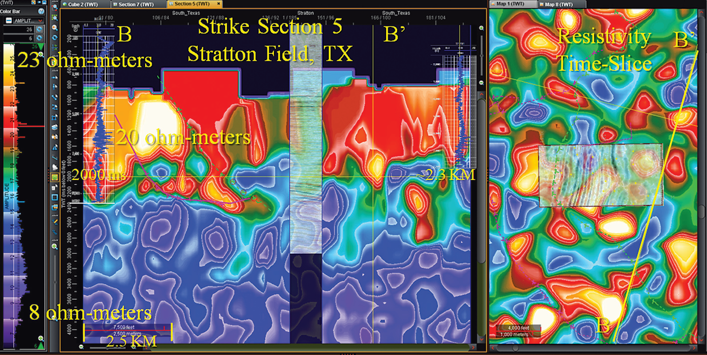
An apparent resistivity cross-section from south-south-west to north-north-east cutting the south-east corner of the Stratton 3D seismic survey is shown below. This cross-section connects two deep resistivity logs, demonstrating how well the 20 ohm-metres recorded on the well log matches the 23 ohm-metres shown on the apparent resistivity colour scale on the left.
We were amazed at how well the 1986 interpretation matched patterns in the apparent resistivity cross-sections. Note there are fewer lightning strikes at low elevations, which means there are fewer shallow control points. The gap at the top of the cross-sections is a result of the assumption relating cloud height to the strength of the strike. The gap between the ground and the base cloud height is reflected in the subsurface as a gap in the data. This gap is where electrical currents in the atmosphere bleed off, and clouds do not generate enough charge to create a recordable lightning strike. Also, fewer low elevation strikes mean the interpolation creates larger extended features in the shallow data and these larger interpolated features of higher resistivity tend to be above certain faults, or at fault boundaries, and are possibly showing diffuse residual hydrocarbons from migration pathways.
This South Texas example shows spatial correlation between faults mapped in a previous publication with apparent resistivity volumes created from the more recent lightning database. Each lightning analysis project Dynamic has done so far has shown similar correlations between the lightning derived maps and volumes and available geological and geophysical control.
There are numerous opportunities for research and exploration with a new geophysical data type: think what could be seen differently in your trend or prospect, with another layer of information sourced by enormous electrical currents.
References:
Franklin’s Lightning Rod, The Franklin Institute.
Nelson, H. R., Jr., D. J. Siebert, and L. R. Denham, Lightning Data – A New Geophysical Data Type, 2013, adapted from extended abstract prepared in conjunction with oral presentation at AAPG Annual Convention and Exhibition, Pittsburgh, Pennsylvania, May 19-22, 2013
The Earth’s Electrical Environment, 1986, Chapter 16, Telluric Currents: The Natural Environment and Interactions with Man-Made Systems, Page 236.
Hutton, V.R.S., 1976, The electrical conductivity of the Earth and planets, Report on Progress in Physics, Vol. 39, No. 6, pages 487-572.
Cagniard, L. (1953). “Basic theory of the magneto-telluric method of geophysical prospecting,” Geophysics, 18: 605-635. doi:10.1190/1.1437915.
Martin Murphy, Vaisala lightning researcher, personal communication, ILDC/ILMC Conference, Wednesday, March 14, 2018.
Almbaugh, D., H. Huang, J. Livermore, M. S. Velasco, (2016) First Break, volume 34, April 2016, p. 65-72.
Thompson, A.H., S. Hornbostel, J. Burnes, T. Murray, R. Raschke, J. Wride, P. McCammon, J. Sumner, G. Haake, M. Bixby, W. Ross, B. S. White, M. Zhou, and P.
Peczak, Field tests of electroseicmi hydrocarbon detection, (2007) Geophysics, Vol. 72., No. 1 (January-February 2007, p.N1-N9, 10.1190/1.1299458.
Labson, V. F., and A. Becker, Natural-field and very low-frequency tipper profile interpretation of contacts, (1987), Geophysics, Vol. 52, No 12 (December 1987) p. 1697-1707.
Ewing, T.E., 1986, Structural Styles of the Wilcox and Frio Growth-Fault Trends in Texas: Constraints on Geopressured Reservoirs: BEG, Report of Investigations, 154, 27-56.