Can sparse OBN equal savings and data quality?

By Yannick Cobo, Rodrigo Felicio, Carlos Calderon and Paul Farmer; ION

Published at: July 18, 2021

Depressed demand for oil and gas due to the pandemic, as well as commitments to honor the goals of the Paris Climate Accord, continue to place pressure on oil and gas companies to decrease costs and capital expense in order to deliver value to shareholders. In exploration, drastic budget cuts took place, limiting exploration to nearfield and lower cost development opportunities. However, to exploit these nearfield opportunities efficiently, high-quality seismic data is necessary. Typically, higher quality seismic is associated with tighter acquisition geometries or acquisition types such as ocean-bottom nodes, in order to capture broader frequency spectra, longer offsets and richer azimuthal coverage. However, these qualities usually come with a higher price. One way to decrease the cost and time of seismic data acquisition is to design sparser surveys by decimating the number of shots and receivers used. To understand the tradeoffs of such decimations, we used ocean-bottom node data from a complex geological setting in a pre-salt play of the Santos Basin, offshore Brazil to compare how different geometries might impact the ability to build accurate velocity models.

Geology

The study area is in ultradeep waters (2 km) of the Santos Basin and the geology is comprised of a 2–4 kilometer-thick sequence of mostly clastic sedimentary rocks overlaying evaporite layers and thick salt comprised mostly of halite, with secondary intervals of anhydrite, gypsum, tachyhydrite and carnalite. These salt layers have a complex structural history and may form massive heterogeneous bodies up to 3 kilometers thick, displaying a complex array of folds, faulting, overhangs and mini-basins. Below these units, the pre-salt is comprised of syn-rift sequences of clastic sediments, basalts, carbonates and evaporites, which include reservoir rocks (Carlotto et al., 2017).

Method

The ocean-bottom node dataset used has approximately 3,000 nodes deployed on a 500m by 500m regular spacing grid, and shots on a 50m by 50m carpet grid. This design yielded rich azimuth data coverage with offsets as long as 27 km, and thus provided an excellent dataset to conduct our analysis.

For this analysis, we tested three scenarios, each representing a different shot and receiver decimation from the original survey, to understand the effects of such decimations for velocity model building with a fully automated workflow. The workflow solely uses full-waveform inversion (FWI) for the estimation of velocities, with the exact same inversion parameters for each scenario. Thus, each scenario utilizes the same initial velocity model which is a smooth model with no information related to the position of geobodies, and the same data-derived source wavelet.

The velocity estimation workflow is comprised of two different full-waveform inversion methods that use a cost function that emphasizes travel time differences between field and synthetic data to help prevent cycle skipping (Wang et al., 2019). For the initial iterations, only first-arrival events were modeled and matched to the real data, an approach akin to that described in the work by Sheng et al. (2006). Once the first arrival or FAFWI converged to a solution for relatively low frequencies, first arrivals and wide-angle reflections were also targeted using travel-time FWI (TTFWI). In TT FWI, a cross-correlation of local time windows was used to estimate the difference in time between the two datasets. Both FAFWI and TTFWI use a hierarchical scheme in frequency, starting from the lowest possible frequencies (<3 Hz) and progressing to a high frequency limit (5.5 Hz), at intervals of 0.5 Hz, designed to gradually build the velocity model from low to high wavenumbers (e.g., Virieux and Operto, 2009). We note that the velocity model building workflow did not include interpretation of high-contrast interfaces such as the top and base of salt bodies, in an attempt to use a data driven approach to model building, based on the high quality, long offset data.

In the first test, we used the original geometry of the OBN survey, nodes distributed on 500m by 500m grid and shots in a 50m by 50m carpet geometry; in the second, nodes were decimated to a 1 km by 1 km grid, while the shots were in a 100m by 300m carpet; in the third, nodes were further decimated to a 2 km by 2 km grid, whereas shots were kept in the same 100m by 300m configuration.

Results

We illustrate the quality of the models obtained for each of the three scenarios above in two ways. First, we compare the models against a higher-grade velocity model (labeled as ‘Final model’). The final model is an accurate and matured velocity model, derived mostly from FWI from diving waves and wide angle reflections in the data, tomography iterations interleaved with subsequent iterations of FWI, and model refinement that used a top of salt horizon and well constraints. This model is not used for estimation of the velocity for the three described scenarios. We compare the migrated stacks obtained from prestackdepth migration of a legacy streamer dataset from the same area for the final model and each of the tested scenarios.

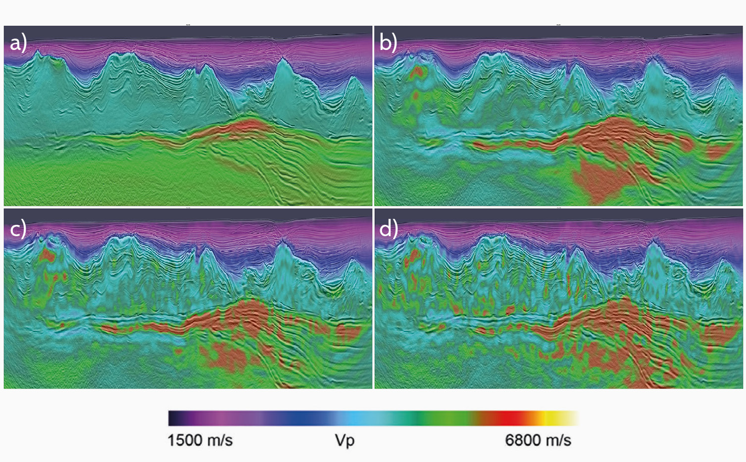
Figure 1: (a) Final ‘reference’ velocity model (b) FWI model for 50 x 50m shot spacing and 500 x 500m receiver spacing; (c) FWI model for 100m x 300m shot spacing and 1 km x 1 km receiver spacing; and (d) FWI model for 100m x 300m shot spacing with 2 km x 2 km receiver spacing. The stack image corresponds to a stack obtained with the final model derived with the dense geometry.

Figure 1 shows vertical sections of the velocity models obtained from the three scenarios compared to the final model. All four scenarios reached similar solutions that converge towards the final model, i.e., all inversions are able to predict the bulk of the salt geometry from the initial smooth sediment-only velocity model. Note also that model resolution decreases as a function of node density. For example, as the node spacing is increased, the cascaded FWI flow recovers a relatively smooth velocity gradient above the top of salt, while introducing undesirable velocity oscillations in both the salt and pre-salt sections, more evident in the case of 2 km receiver spacing. Thus, decreasing the number of nodes by an order of magnitude or more leads to ‘noisier’ solutions that require a more aggressive model regularization.

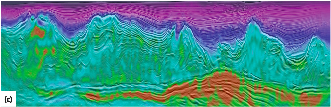
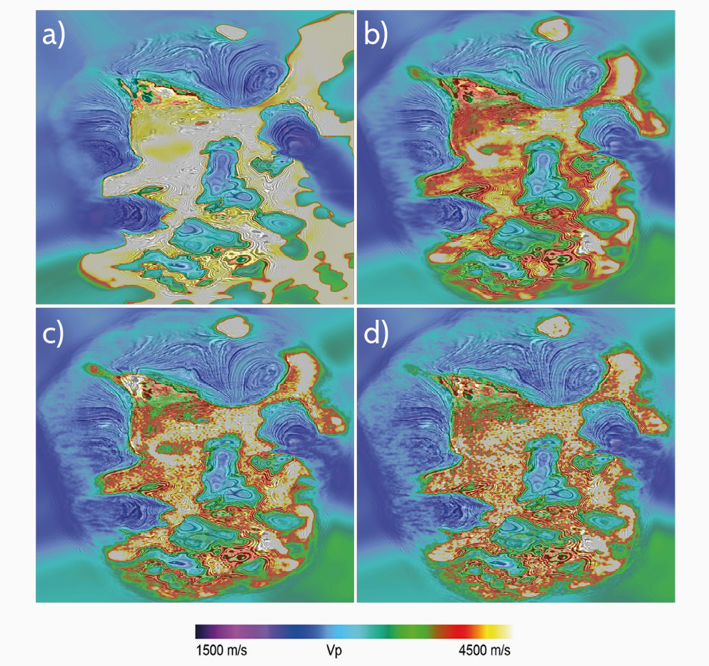
These observations are further corroborated by inspection of depth slices presented in Figure 2. Delineation of salt bodies (velocities of about 4500 m/s, i.e., reddish to white colors in the figure) and mini-basins are comparable to those observed from the final model (Figure 2a), but with model degradation as the nodes become sparser. The model derived from the 1 km node spacing provides a good compromise relative to the 500m result and the oscillatory nature of the 2 km node result.

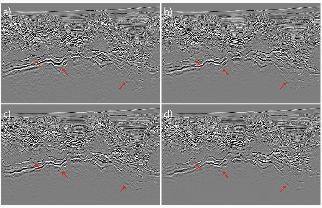
Figure 2. Depth slices below top of salt of velocity models for (a) Final model; (b) 50 x 50m shot spacing and 500 x 500m receiver spacing; (c) 100m x 300m shot spacing and 1 km x 1 km receiver spacing; and (d) 100m x 300m shot spacing with 2 km x 2 km receiver spacing. The stack image corresponds to a stack obtained with the final model derived with the dense geometry.

Vertical sections of migrated images with a maximum frequency of 45 Hz for the models are shown in Figure 3. These migrations use a narrow-azimuth streamer dataset acquired over the same area as input, to evaluate the quality of the inverted models. In these comparisons, we observe the progressive loss of resolution of salt bodies and mini-basin delineation with sparser geometries resulting in a gradual pushdown of the top of salt events. We also note in the Figure a decrease in focusing and continuity of events marking the base of salt and pre-salt section, particularly beneath the mini-basin on the right side of the sections. Despite this decrease in resolution of the model, the result for the 1 km node spacing is very comparable to the model image derived from the 500m by 500m node spacing.

Figure 3: Kirchhoff PSDM stacks of streamer legacy data for (a) production model and the FWI-derived models with node grids of (b) 500 x 500m, (c) 1 km x 1 km, and (d) 2 km x 2 km.

Velocity model building conclusions

The velocity estimation results presented show that sparse node surveys in general produce poorer velocity models than relatively denser ones when deriving the model from FWI with primarily diving wave energy. However, a relatively coarse source-receiver distribution is still able to produce a high quality velocity model. In our particular case (OBN survey in ultradeep water), we find that receiver sampling of 1 km by 1 km and a shot geometry of 100m by 300m spacing is a viable alternative to denser node surveys with four times more nodes and six times more shots when estimating the velocity model from large offsets and low frequencies.

Practical conclusions

Pre-salt exploration within the Santos Basin presents unique challenges because of the complex geological settings with deep targets, massive heterogenous salt bodies, and a complex array of structural features. Several recent ocean-bottom seismic (OBS) surveys have been acquired over fields within the Santos and Campos Basins with the aim of providing superior images for reservoir characterization and development. The reasons for superior imaging achieved by OBS data compared to towed streamer data are well understood and include extended bandwidth – particularly at lower frequencies, improved signal-to-noise, longer offsets, and full azimuth.

The application of full waveform inversion (FWI) to OBS datasets has proven highly successful for improving the velocity model – leading to superior imaging results. However, the survey effort required for a conventional OBS survey is still significant in terms of both its cost and duration. Consequently, OBS surveys are commonly limited to specific field appraisal and development objectives.

The decimation exercise described demonstrates that an improved and reliable velocity model can be derived from a ‘sparse’ OBS survey configuration. Deploying fewer receiver nodes at increased intervals and increasing the source sail-line separation can deliver significant efficiencies and allow an OBS deployment to be adapted for larger exploration-style surveys. Sparse OBS configurations do limit the imaging quality because of spatial aliasing and reduced signal-to-noise when compared to a conventional OBS dense survey; however, integration with legacy narrow-azimuth (NAZ) towed-streamer seismic data can provide significant uplift in imaging for the exploration process. NAZ streamer-data provides the well-sampled input data for imaging, particularly in a shallow-to-intermediate depth range, while the ‘sparse’ OBS data provides more reliable velocity updates that are crucial for improved deep imaging and potentially an improved pre-salt image.

Utilizing the traditional approach of NAZ streamer data, but refreshing the earth model with the use of high quality, but sparse, OBS data, will allow improvements in the overall quality of the final image at a fraction of the time, effort, and cost. Therefore, not only can early OBS-adoption during the exploration cycle provide a viable alternative in complex geologies, such as the pre-salt plays in Brazil, but in the longer term or further down the oilfield lifecycle, these ‘sparse’ surveys may also provide a baseline for future high-density infill for reservoir development as well as 4D-monitoring surveys.

The global energy sector from a subsurface perspective