A simple guide to the parameters involved in seismic depth conversion – a complex but important subject in geophysical seismic processing.
Why Do We Use Depth Conversion?
Seismic reflection data records the two-way travel time (TWT) to a reflection event from the surface. Depth conversion is the process by which interpreted seismic horizons (and time domain seismic itself) are converted from the travel time domain to the depth domain. (Note that depth migration is a seismic imaging technique that improves reflector positioning. Depth migrated data is often converted back to time and then depth converted conventionally as this gives greater flexibility for testing alternative velocity models.)
Depth conversion can be simple or complex. Approaches to the technique vary all over the world and are dependent on the play scenario and geological overburden. Depth conversion is a big, technical topic for a short article, so we are going to try to make some general comments and highlight a few points that are perhaps less widely known.
When predictions of depth values are made at multiple regular points on a grid pattern then we tend to view the result as a depth surface. Smooth, best estimate predicted depth surfaces of this type are used for multiple purposes including drilling prognosis (well forecasts), in-place hydrocarbon volume estimation (surfaces) and reservoir modeling (surfaces).
The standard practice use of depth surfaces for making depth prognosis for well targeting purposes is entirely valid. However, the use of the same surfaces for in-place hydrocarbon volume estimation is not valid. A discussion of this and the role geostatistics plays in addressing this problem was given in a previous article ‘A Simple Guide to Volumetrics’ (GEO ExPro Vol. 12, No. 3).
Understanding Rock Velocity
To convert time reflections to a depth surface we need to know the velocity. The depth is then estimated from the simple geophysical relationship that depth = velocity x time.
The velocity of a rock is a fundamental physical property related to its hardness. As a simple rule of thumb, if you hit a rock with a geological hammer, fast rocks go ‘ding’ and slower rocks ‘thud’ (or even ‘squelch’!).
For depth conversion, velocity varies with rock type, depth of burial and pore space factors such as porosity and the presence of microfractures. In general, the slowest velocity we encounter would be sea water, which is typically 1,500 m/s. The fastest velocities we commonly come across would be the matrix velocity of rocks such as sandstones, limestones and dolomites and igneous rocks, where the velocity reaches 6,000–6,500 m/s.
Determining Rock Velocity
Velocity measurements come from a variety of methods but the three most important sources for depth conversion are:
- Seismic processing velocities
- Sonic logs from well data
- Checkshot and VSP surveys, also obtained from wells.
- Seismic Processing Velocities
Seismic processing velocities in their most basic form are the so-called stacking velocities. Seismic processing requires curving events on gathers to be flattened using the NMO stretch correction before they can be stacked. The stretch factor is related to the RMS average velocity and so NMO correction gives an estimate of the velocity profile at each point it is picked in the dataset. The stretch factor is small for deep events and increases in magnitude for shallow events.
Wells give us depths to geological markers and by tying a well to the seismic using a synthetic seismogram the seismic time events that are interpreted can be related to the geology. A well depth and a seismic horizon time to the same event can be used to define a so-called pseudo-velocity and these are often used in depth conversion.
Checkshot & VSP Velocities
Well velocity information is obtained from both checkshot data (or better, from more detailed VSP survey first arrival times) and from sonic logs. Checkshot and VSP surveys give direct measures of both average and interval velocity by recording the travel times and depths from surface to a series of geophone locations along the length of the well.
Sonic Log Velocities
Sonic logs are calibrated using checkshot data, resulting in the calibrated velocity log (CVL). The CVL is the best velocity information we have and combines the benefits of checkshots and sonic log data.
Without well information the only source of velocity data is through the seismic processing accompanying seismic reflection data. Seismic velocities have some useful characteristics – for example, they cover the survey area with relatively dense sampling. Unfortunately, seismic velocities are potentially inaccurate, insensitive to velocity changes in deeper layers and noisy. Because of the noise, seismic velocities should be filtered or smoothed before use. Kriging using an explicit nugget (noise) model is a good choice for this task.
Seismic velocities can be used as an average velocity to a horizon for single layer depth conversion, or the Dix formula can be used to convert to interval velocities for use in a multi-layer depth conversion. Seismic velocities are inaccurate (biased) and can over- or underestimate the actual velocity by as much as 10–20%. Resultant depth prognosis will have similar error magnitudes, but the uncertainty in gross rock volume (GRV) is less affected by bias in the velocity field than it is by local variation and so the GRV uncertainty will be less affected.
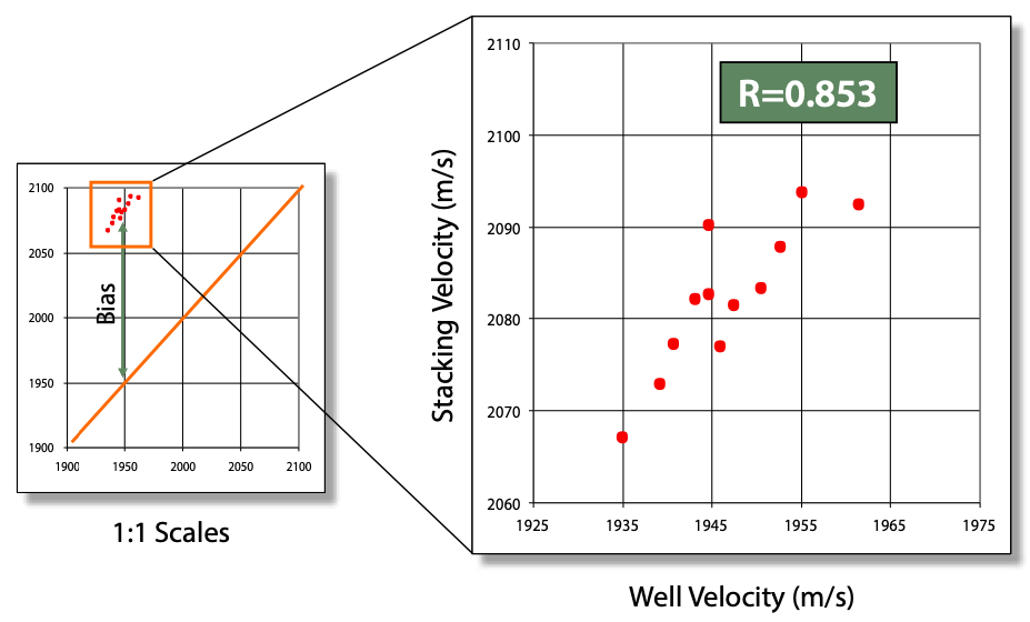
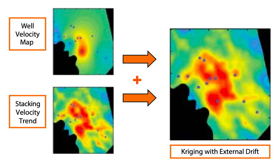
If well data are also available, then seismic velocities can be calibrated and used to provide regional trends away from well control. This can be done geostatistically using methods such as kriging with external drift or collocated co-kriging. Alternatively, a simple linear regression calibration can be used. Figure 1 shows a comparison and calibration of seismic velocity to well data and Figure 2 shows the combination of both data types geostatistically.
The value of using seismic velocities diminishes quickly as the depth (or time) to targets increases due to poor velocity sensitivity to deeper reflections. The importance of seismic velocities also diminishes as more well control becomes available. Although useful, seismic velocities are the lowest quality source of velocity information for depth conversion.
Using Well Velocities
Well data are usually very sparse and cover very little area in a regional depth conversion. For this reason, well information is often used to define functions that relate the interval velocity behavior to the regional trends in the geology. There is a very rich family of functions available to choose from, but the most popular approaches are:
- Constant interval velocity
- Well velocity maps
- Depth/time functions
- Velocity/time functions
- Velocity acceleration functions
Some forms of velocity functions and, in particular, linear acceleration functions of the form V0+kZ (where V0 = reference velocity, k is the velocity gradient, and Z is depth) are very dear to the heart of many a geophysicist. There are sound reasons for their use, but some of the associated practices have become rather prescriptive and should be re-considered.
The first point to make about V0+kZ velocity functions is that they are strictly linear. This is both good and bad. Good because they avoid the bias of using average well velocities from the crest of a structure to depth convert a flank where the velocity might be expected to be higher due to compaction; bad because compaction effects are not linear and so velocity functions can become non-physical quite quickly outside of the depth range of the data from which the function was derived. For this reason, it is good practice to examine proportional horizon slices through the instantaneous velocity field at different levels within the layer to check the velocities are not physically too high or too low.
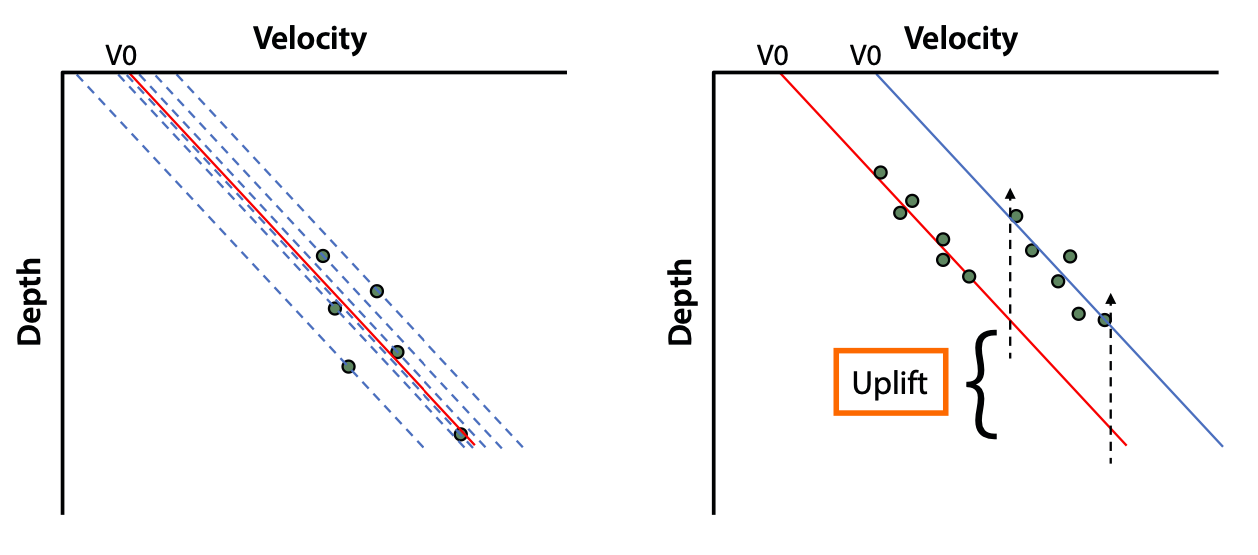
Another problem lies in a popular practice of (typically) calculating a global gradient k from a group of wells and then backing out an apparent V0 at each well. The V0 values are then over-interpreted by the geophysicist as a physical parameter whose spatial pattern represents differences in burial history (typically uplift). As well data are sparse and noisy this is almost certainly an over-interpretation and is usually just regression of noise. Only if groups of wells exhibited different V0 (for the same gradient k) might an uplift interpretation be justified (Figure 3). In general, V0 mapping methods are usually just error residual corrections in disguise and should be avoided.