Surface Geochemical Exploration
A newly developed method for detecting petroleum seepage using surface geochemical exploration.
Changes in the physical and chemical properties due to petroleum seepage. © ORG Geophysical AS
The use of surface geochemical exploration methods is based on the concept that all petroleum accumulations suffer some leakage to shallower intervals and eventually to the surface.
This leakage can be detected directly by sampling and analysing the petroleum compounds in surface sediments, the water column or in air.
The seepage process can also cause changes in the mineralogical and environmental conditions, which can be detected using a range of other chemical, physical and microbiological methods.
In recent years, the most commonly used approach to surface geochemical exploration in offshore areas has been the collection of gravity core samples that are then taken ashore for analysis of any petroleum components in the sediment. In deeper water (>100m), collection of gravity core samples can lead to the loss of light components due to the pressure drop experienced when moving the core to the surface. The onshore analysis of the sample material means that results are often available only 6–8 weeks after completion of the sampling cruise, which can be a concern in an exploration project.
The New System Using Sub-Sea Units
How The New System Works
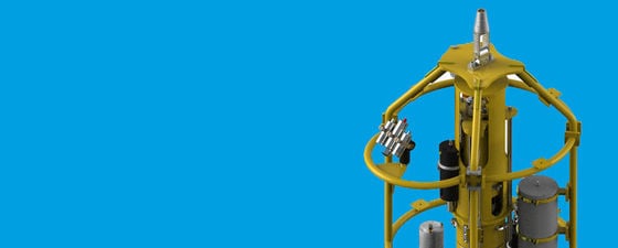
The two-metre-high sub-sea unit is equipped with sensors for measuring environmental parameters and the analysis of polyaromatic hydrocarbons.
To mitigate some of the weak points of the gravity core approach, ORG has developed a new approach in recent years. It is based on a sub-sea unit (SSU) equipped with a pump, camera and a range of sensors for environmental analysis and the detection of polyaromatic hydrocarbons (PAH).
The SSU is lowered onto the seafloor and pumps a sediment suspension through a closed system up to the vessel, where the flow is passed through a silicone-membrane gas filter and the released material is analysed by a selected-ion flow-tube mass spectrometer (SIFT-MS) with a cycle time of approximately two seconds.
A sample of the pump flow is passed through several sensors on the SSU for measurement of environmental and PAH parameters.
Measuring Hydrocarbon Concentrations
The mass spectrometer measures and reports the concentrations of C1–C12 hydrocarbons in the gas from the gas filter. Obviously, the sensitivity of the method will be strongly controlled by the compound solubility in water and the efficiency of the gas filter in extracting the hydrocarbons from the water. Further testing is underway to optimise this transfer.
Continuous Data Collection
Operation principal: Data collection scheme.
The mass spectrometer and the environmental sensors collect data continuously, starting when the vessel arrives on position with the SSU suspended about 10–15m above the seafloor and pumping only sea water. Data collection continues after it has been lifted from the seafloor during transit to the next sample location. To reduce this very large dataset to more manageable numbers, average data values have been calculated for several time intervals and these have been compared in order to find the most representative values. Some of these intervals cover the time during which the SSU is positioned on the seafloor, while others represent time when the unit is suspended in the water column close to the bottom and pumps only water.
The vessel is also equipped to collect gravity cores, which can be used for a broad range of chemical and microbiological analyses. The sediment material in the suspension flow can be collected on board the vessel for later analysis. Tests are ongoing to evaluate if this material is equivalent to sediment samples from gravity cores.
Geochemical Surface Exploration in the Norwegian Continental Shelf (NCS)
Project areas on the Norwegian Continental Shelf shown in yellow.
After some small-scale test projects in 2016, the system was operationally deployed in 2017, collecting data in seven different areas on the Norwegian Continental Shelf (NCS), with a total of over 1,500 measured stations. Project areas ranged from the Central Graben up to the Barents Sea, covering areas that have very different deep and shallow geology. These differences in geological setting can explain some of the variations that were observed, but there were also several common aspects in all the projects.
A comparison of different areas along the Norwegian Continental Shelf shows significant variations in the measured hydrocarbon concentrations. These variations are probably due to differences in the deep and shallow geology. It comes as no surprise that the highest concentrations come from places where active petroleum generation is ongoing at present.
Comparing Average Hydrocarbon Concentrations
Methane distribution in different projects on the Norwegian Continental Shelf stretching from the Central Graben up to the Barents Sea. Note the significant variation between the different areas.
When comparing average hydrocarbon concentrations in the various sediment intervals with those from the water intervals, the values turned out to be very similar. While this correspondence was unexpected, it was observed in all measured components and in all the areas that were covered.
Two factors are thought to account for this similarity:
Firstly, to pump the sediment material up to the vessel, a certain volume of additional water is required to achieve a good flow. The exact volume of this excess (sea) water is not known but it can significantly dilute the sediment material, so the resulting hydrocarbon concentrations will be a combination of sediment and water values. The system is currently being modified to better constrain this dilution.
Secondly, there is no reason why hydrocarbons seeping from the deep subsurface into surface sediments should remain there. In fact, seepage is expected to continue into the water column. As such, it is not surprising to find similar hydrocarbon concentrations in the water and in the sediment interval.
Average n-butane concentrations measured during a 10-minute period while pumping a sediment/water slurry (left) and a 5-minute period while pumping sea water before the sub-sea unit is positioned on the bottom. Reported values represent concentrations in the gas flow from the gas stripper. The map area measures 17 by 10 km and contains an oil and gas discovery (hatched outline).
Both sediment and water data show geographical clusters of stations with anomalous measurement values. This gives added confidence to the assumption that these reflect real variations in the amounts of hydrocarbons present in the top sediment and in the water column close to the bottom.
It appears that bottom currents do not effectively mix the water close to the sediment surface, at least not in the areas that were measured.
Comparing Known Accumulations & Untested Prospects
Known Accumulations
The effectiveness of this method in identifying subsurface hydrocarbon accumulations can be assessed by evaluating the surface expression of known discoveries. Once more, there are significant variations between different areas: in one area all known accumulations are accompanied by anomalous hydrocarbon concentrations at the surface, while in other areas up to a third of the known discoveries are ambiguously detected in the surface measurements. The ‘false negatives’ can sometimes be explained, for example, by a lower pressure in the discoveries or a different nature of the (near) surface sediments, but further work is needed to better constrain this.
Untested Prospects
Methane concentration data over an undrilled structure (dense part of the grid) compared with tightly sampled calibration wells with shows or discoveries (area enlarged in separate boxes). The map area measures 27 x 49 km; the radius of the sample circle around the calibration wells is approximately 250m. Methane concentrations are expressed as ppb in the gas from the gas stripper.
An example of how the surface measurements can be used to evaluate the petroleum charge risk of a given prospect is shown right. An untested prospect was densely sampled (central part of sample grid) and the resulting measurements show no significant anomalies over the structure, neither in the light components (gas indications; methane concentrations shown in the figure) nor in the heavier components (oil indications). Nearby wells with discoveries and shows were tightly sampled for comparison and do show multiple anomalous values. Given the shallow burial depth (<1 km), the lack of surface anomalies meant that the charge risk for this prospect remained unchanged.
Based on the results from the 2017 projects, the new method has shown to accurately measure hydrocarbon concentrations in surface sediments and in the water column. Significant variations in the measured amounts are seen both within and between different areas on the Norwegian Continental Shelf and the results can help to better constrain the charge risk of undrilled prospects.
At the same time, the occurrence of clusters with anomalous hydrocarbon measurements is by no means well understood. Further work is needed to investigate the effects of changes in the deep geology and environmental variations in the shallow layers.
The lack of contrast between measurements in the sediment interval and in the water column suggests that it may be better to limit data collection to the water column in future projects, possibly as a first phase, before zooming in on the most promising areas.