The Value of Monitoring Fractures
Real time frac monitoring shows the progression of fractures opened during the fracking process, knowledge which can impact drilling decisions.
Unconventional reservoirs are a growing part of the oil and gas industry in Latin America. New technologies, new tools and new understanding of the geology are necessary to properly develop these reservoirs, as international operators are faced with the challenge of understanding and applying technologies that do not have any clear analogues in conventional reservoir development. A major part of the development of these rich reservoirs is hydraulic fracturing.
Hydraulic stimulation or fracking is one of the most prominent and important of these technologies, and has played a pivotal role in enabling the economic production of hydrocarbons from shales and other low permeability formations that comprise the unconventional space. By creating new permeability pathways and enhancing pre-existing ones, this technology exploits fractures to extract hydrocarbons from formations that would otherwise be uneconomic. Assessing the effectiveness of fracking operations requires an understanding of the fracture network created or activated by the stimulation, as well as of how those fractures develop. It is this ‘how’ question that real time fracture monitoring is designed to address.
The number of fracture-stimulated wells in Latin America is on the rise and the case study in this article is an excellent example of the quality and importance of the data that can be attained using state-of-the-art technology.
Real Time Fracture Monitoring
Real time maps of the fractures being opened during pumping are required so completion engineers can improve their fracking projects. Monitoring the progression of fracture development in real time provides the information that they require.
The Seismic Emission Imaging method is used to create real time images of the fractures. For frac monitoring, grids of geophones are distributed on the surface or buried in shallow wells. The signals received by these geophones are recorded continuously for the duration of the frac project. Microseismic recordings from these grids are used to directly image the fracture networks that are activated by the pressure changes caused by the frac pumping, as they open new fractures and cause movements along pre-existing ones. The opening of the fractures in the rock causes seismic waves to be generated, which propagate to the recording array at the surface. The recorded seismic waves are imaged over many time windows to create a large number of seismic emission volumes, which are integrated for over large time intervals, with the final volume being the result of many minutes or hours of integration.
Dynamic Reservoir Response
The rock movements at any location in the rock are discontinuous and episodic. During pumping, fractures are opened in varying directions and at progressively larger distances from the frac point. Continuous imaging of the volume for seismic emissions allows the progression of the fracture development to be mapped in real time. This is called Time Lapse Seismic Emission Imaging. The images of the seismic emissions are output at short time intervals, which allows the progression of the fractures to be monitored in real time.
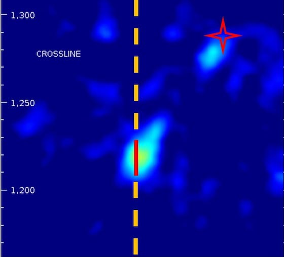
A. Activity at the beginning of stage 3: high activity at the perf location along the well that is being fracked, and some activity at the nearby well.
B. Formation breakdown occurs 20 minutes into stage 3 pumping, with a fracture activated in a nearby well within a three-minute interval
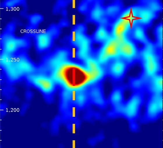
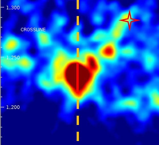
C. Activity continues for 70 minutes near the perf location and in the fracture to the nearby well.
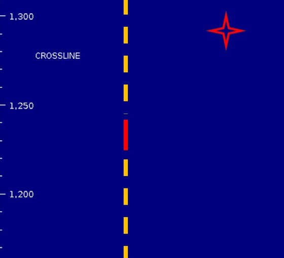
D. This period of active rock movement was followed by an hour of quiet time during which there were no seismic emissions.
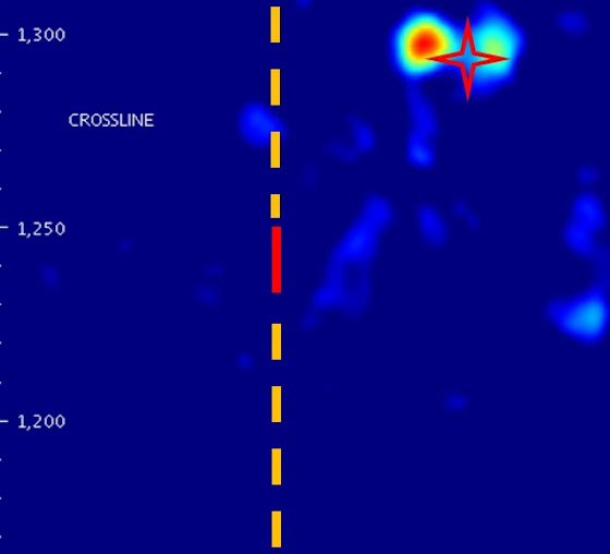
E. Stage 4 commences: activity shows that the nearby well is being fracked but there is no activity at the perf location.
In the example shown here, time lapse imaging shows the frac process from the beginning to the end of pumping for stage 3 of the frac project. The first 20 minutes of pumping shows the desired behaviour in the rock fracturing, with seismic emissions coming from the locations of the perfs (A). After 20 minutes of frac pumping, the passive imaging shows very large amplitudes of seismic emissions that last for about 3 to 5 minutes (B). During this very short period of time, the images show a fracture opening from the frac point in the well propagating to a monitor well 2,000 ft (600m) from the frac point. This fracture was confirmed at the distant well, when monitors in that well detected frac fluid during stage 5 of the frac project. The activity recorded by the geophones and imaged by the processing shows that the fracture that was opened had active movement for approximately 70 minutes after the time of the initial opening (C). This period of active rock movement was followed by an hour of quiet time during which there were no seismic emissions (D), after which small movements in the rock along the fracture were reinitiated. The frac pumping was ongoing for the entire time.
The animation for stage 3 illustrates the real time activity that could be provided to the completion engineer. This example indicates that the rock movement during and after the fracture opening relieved the stress in the rocks; as pumping continued, the pressure in the fracture built up until it reached a level at which the stress increase caused additional movements along the fracture.
Stage 3The final frame (E) shows the type of activity that was dominant during the frac for stage 4. Pumping continued to fill the very long fracture with fluid and the pressure increase at the well 2,000 ft away caused the rocks at that location to be extensively fractured. During this stage, rocks at the frac pumping location were not fractured, while the rocks at the distant well had extensive induced fracturing. The animation for stage 4 illustrates how real time monitoring would have provided this information to the completion engineer and the completion plan could have been modified. Instead, the frac project was stopped only after the damage had already been inflicted.
Stage 4
Fracture Imaging
Using the emission volumes for selected time intervals, fractures that are opened by frac pumping can be mapped. The final figure (F) shows a fracture network that was mapped using the data from about 10 minutes of recorded data. The emission volumes for this period were integrated to form a single emission volume. The passive emission volumes are combined using a suite of tools that include the statistical and graphical analysis for noise editing and threshold application to remove the background, and the fracture volumes are computed from the combined passive emission volume. The volume is collapsed to fracture surfaces automatically using a patent-pending algorithm (Geiser and Vermilye, 2011).
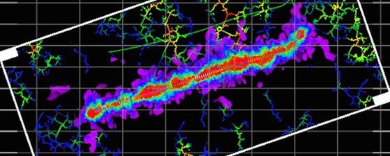
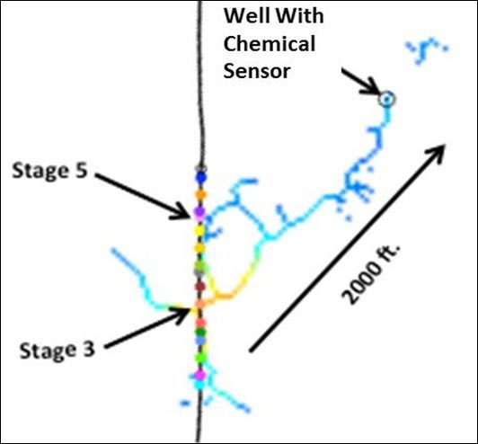 F. A Tomographic Fracture Image (TFI) was computed using the data for the few minutes covering the time of formation breakdown.The Tomographic Fracture Image (TFI™) shown in this figure is very complex. It passes through the frac point, through the distant well, and also wraps around and crosses the well being treated at the frac points for stages 4 and 5. This shows that the large fracture from the well being treated to the distant well was open before the pumping started for those stages, which explains why pumping for stages 4 and 5 could pass the pumping pressure to the distant well during the entire pumping time. We interpret these observations as follows: as the fluid pressure in the fracture reduced the effective stress and hence the friction, the fracture became seismically active until the stress was relieved. Subsequent pumping drained into the region around the offset well until enough fluid moved into the well to cause a pressure kick and chemical tracer detection. The time lag may be explained by the time required to both pump up the pressure in the fracture system between the wells and to compensate for leak-off into the rock mass. Stage 3 was completed without knowledge of this major fracture opening because the treatment fluids did not arrive at the nearby well until stage 5 and real time, time lapse imaging was not available to the completion engineer.