Seismic reservoir characterization with efforts at quantitative interpretation: a case study
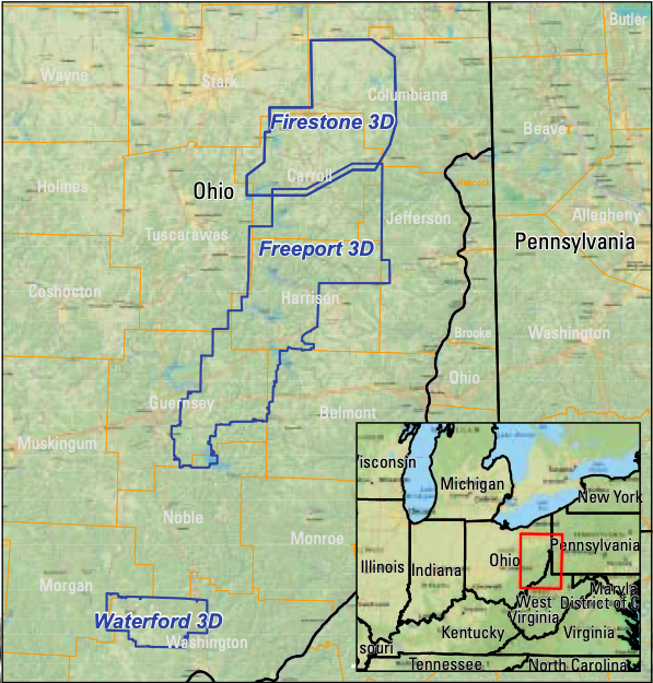
Eastern Ohio has become a new drilling target and the focus of development activity in the Utica Shale play. Thermal maturity studies of the Utica Play Shales have indicated a north-east to south-west trend over eastern Ohio and western Pennsylvania, with a western oil phase window, (Mariani, 2013). The Utica Play thins to the west in Ohio and becomes deeper and thicker as its dips to the east and south-east of the Appalachian Basin (Antoine and Frederic, 2016). In eastern Ohio, therefore, the Utica Play is the preferred target (over the Marcellus) due to its increased thickness within the oil and wet gas windows and the higher reservoir pressures present because of the extra 2,000–6,000 ft (610–1,830m) of burial.
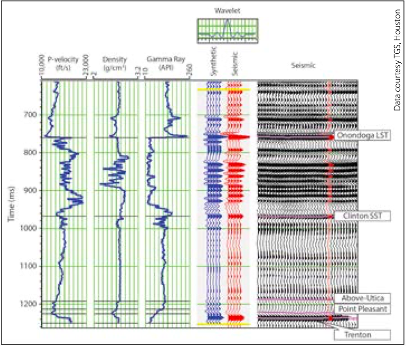
In this case study, we present our attempts at reservoir characterization of the Utica–Point Pleasant package in eastern Ohio, with the goal of identifying sweet spots. Such an exercise entails understanding the elastic properties, lithology, fluid content and areal distribution of the reservoir intervals. A good starting point for this is to use well data and understand the parameters that populate the reservoir intervals at the well locations, so sonic, density, gamma ray, resistivity, and porosity log curves were sought for the available wells within the 3D seismic volume. Core analysis results, geochemical as well as geomechanical data, were available for one well.
Preparing and preconditioning seismic data
As we started compiling well data for our study, we realized that the wells with density logs were located in a cluster to the northern part of the survey, and very few wells had sonic and density curves, which is unfortunately a frequently encountered situation. It is always desirable to have a uniform distribution of wells with sonic, density, and other curves, even if sparse, because it helps the generation of a reliable low-frequency impedance model for impedance inversion, as well as for carrying out any neural network analysis for computation of a reservoir property. Once the final seismic data were loaded on the workstation, we assessed the quality and frequency content. The data were preconditioned for random noise attenuation by applying structure-oriented filtering (Marfurt, 2006; Chopra and Marfurt, 2007).
The pre-stack seismic data were preconditioned carefully, making sure that amplitudes were preserved. This entailed supergathering (3 × 3), bandpass filtering random noise attenuation, and trim statics processes, with difference plots taken at each step to ensure that no useful signal leaked through the processes. The angle of incidence information was extracted from the velocity model generated for carrying out simultaneous inversion and overlaid on the offset gathers (below) to help quality control the range of angles that can be meaningfully used in the inversion process. We found that the usable angle range for simultaneous inversion was 34°.
In simultaneous pre-stack impedance inversion, multiple partial angle sub-stacks are inverted simultaneously. For each angle stack, a unique wavelet is estimated. Subsurface low-frequency models for P-impedance, S-impedance, and density-constrained with appropriate horizons in the broad zone of interest are constructed. The models, wavelets and partial stacks were used as input in the inversion, and the output was P-impedance and S-impedance. Because the usable angle range was only 34°, the density attribute could not be determined with simultaneous inversion, which requires angles beyond 40°.
Identifying Shale Play Sweet-Spots
The main goal for shale resource characterization is usually the identification of sweet spots – pockets in the target formation that exhibit high TOC content, porosity and brittleness, thus representing the most favorable drilling targets. The organic richness in the shales influences properties such as P- and S-wave velocities and density (Chopra et al., 2012). In this study, we have tried to bring in data from core analysis, as well as geochemical and geomechanical analysis, and integrate that with surface seismic data. When density and TOC measurements made on the core samples were cross-plotted, a strong linear relationship was seen in the Point Pleasant interval, suggesting that the density attribute would be required if the organic-rich zones in this interval are to be determined from seismic data.
In addition, as the angle range was not favorable for computing density from seismic data through simultaneous inversion, we turned to neural network analysis for this task. We decided to determine density with probabilistic neural network analysis using some of the attributes determined from simultaneous inversion (for further details see http://info.tgs. com/utica-pointpleasant_casestudy). Once the density volume was quality checked and determined, the relationship between density and TOC determined from core data was used to transform the predicted density volume into a TOC volume.
Realizing that the Point Pleasant interval has high calcite content (Patchen and Carter, 2012), meaning its ability to fail under stress and sustain fractures must be high, we extracted the P- and S-wave impedance derived from simultaneous inversion and density derived from probabilistic neural network analysis to compute the Young’s modulus and Poisson’s ratio attributes for the seismic volume. These were then cross-plotted for just the Utica to Trenton interval, which we interpret as prone to fracturing under stress. Its ability to sustain fractures in a relative sense can be examined based on the Young’s modulus attribute.
To examine the lateral variation in the Young’s modulus, we extracted a horizon slice from the Young’s modulus volume. Thus, by restricting the values of the Poisson’s ratio and examining the variation of the Young’s modulus, we were able to determine the variation in the brittleness of the Point Pleasant interval.
Examination of the available XRD data showed that quartz, calcite and clay are the main minerals present in the Utica play. Additionally, regional petrophysical modeling carried out for the condensate region revealed a strong relationship between clay volume (Vclay) and the neutron porosity minus density porosity (NMD) data. Furthermore, the quartz and carbonates groups showed a strong relationship with the neutron porosity curve (NPHI). Thus, if we are able to compute the volumes of neutron porosity and density porosity (DPHI) we should be able to compute the mineralogical content of the Utica play. We therefore crossplotted both neutron porosity and density porosity with those attributes from well log data that could be seismically derived, e.g. P-impedance, S-impedance and density. We found a good correlation between P-impedance and NPHI and density as well as DPHI and we can use these respective relationships for deriving both NPHI and DPHI volumes from P-impedance and density volumes.
A similar analysis was carried out for the Utica interval and we noticed a good correlation between DPHI and density, but a better correlation for S-impedance and NPHI. These determined relationships were then used for deriving NPHI and DPHI volumes from inverted P- and S-impedance and density and to transform the inverted volumes (P-impedance, S-impedance and density) into individual mineral content volumes. It was noticed that more than 40% clay content exists in the Utica interval, decreasing as we go from Utica to Trenton. Quartz group content varies from 20 – 40% for Utica and Point Pleasant intervals, being higher in the former than the latter. Additionally, carbonate content decreases moving from the Trenton to Utica interval. Considering the importance of brittleness and its association with mineralogical content of a formation, we also concluded that mineralogical BI proposed by Jin et al. (2014), would be a useful area of study due to high carbonate content in the target formation.
Seismic Reservoir Characterization of The Point Pleasant Formation
Having characterized the Point Pleasant Formation in eastern Ohio using 3D surface seismic and its integration with core, geochemical, and geomechanical data, we found that it does not seem to follow the commonly found variation in terms of low Poisson’s ratio and high Young’s modulus for brittle pockets. By restricting the values of the Poisson’s ratio and examining the variation of the Young’s modulus, we could determine the brittleness behavior within the Utica and the Point Pleasant intervals based on the mineral content within these formations. Combining the brittleness behavior with the organic richness determined through the TOC content, we could pick sweet spots in the Point Pleasant interval that match production data. This case study demonstrates that the integration of 3D surface seismic data with all other relevant data can be used to accurately characterize reservoir features.