
Applying a “Minimum Economic Field Size” (MEFS) to your prospect assessment is a key process in quantifying the probability of finding hydrocarbon accumulations of a volume large enough to develop economically. However, the way this is handled in companies often leads to confusion, especially when there are multiple fluid phases or multiple prospects involved.
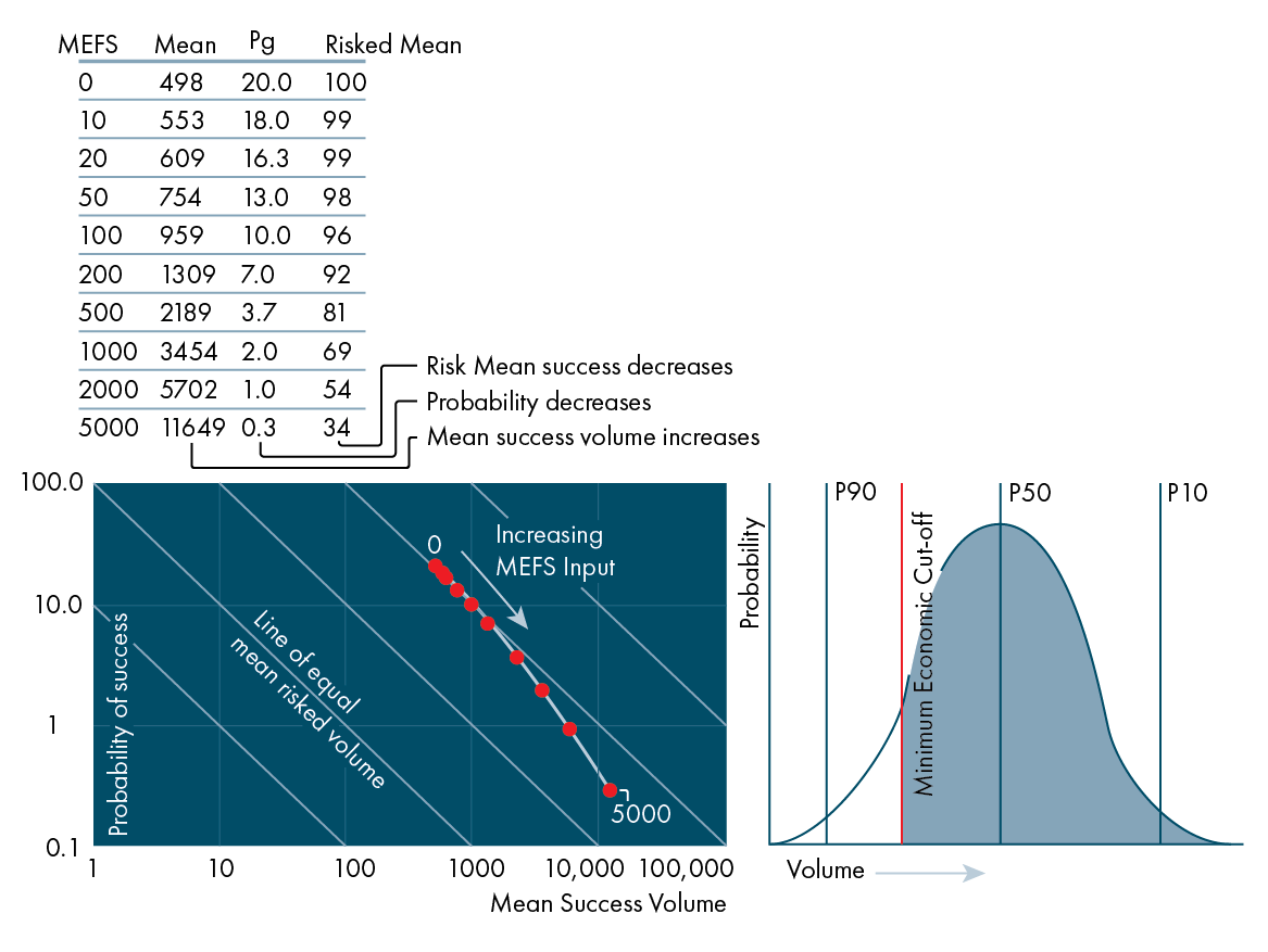
But even the case of a single prospect in which only oil is expected, the simplest example that we can look at, is something worth getting your head around first. As shown in the illustration below, it is particularly important to be aware that applying a volume cut-off will always lead to the Mean Unrisked volume to increase in comparison to the non-truncated case. The reason for this is simple; as one discards the Monte Carlo scenarios where the volume is less than the cut-off, the remaining scenarios will return a higher mean volume.
At the same time, the chance of “commercial” success (Pc) comes down with respect to the non-cutoff case, because there are fewer scenarios in which you will find the field size (or greater) that you hoped for. These two opposing changes do not “balance out”, and the risked mean value will change – typically as shown as a decrease with increasing cut-off volume along the line shown in the plot below.
The real world is often more complicated than single phase prospects. For instance, many prospects have both material oil and gas volumes. That means two cutoffs need to be applied concurrently to get a true insight into the probability of a commercial outcome; one for the oil and one for the gas, because gas is typically worth less than oil. In this case, you need software that can input these two values in one evaluation to get the overall commercial result.
A similar real-world challenge is when there is material condensate volumes with the gas and the user wants to apply a liquids cut-off (oil plus condensate) threshold. So, in summary cutoff’s can be tricky in many situations and in many cases two separate inputs are required but in all cases the output risked mean values will change.
Aggregating targets
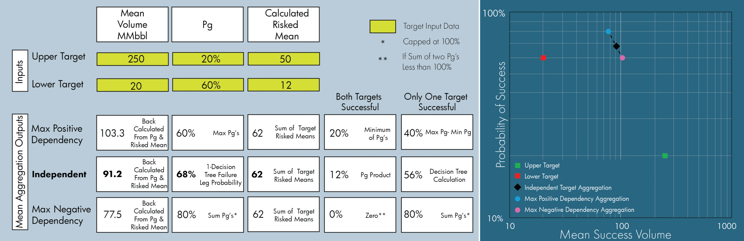
Frequently, explorers are surprised by the outputs from a Monte Carlo process when aggregating two targets. The trick to understanding the outputs of this process is to know that the mean of the aggregation calculation is equal to the sum of the risked means of the targets. This value will not change when dependency between the targets (positive or negative) is applied, as shown in the example below.
It is also easy to calculate the maximum positive and negative dependency cases for the two target aggregation. The shape of the stochastic output will change with dependency, but all outcomes will have identical mean values. The larger numbers that people like to see have been preserved in the Monte Carlo process – nothing has been lost in the stochastic aggregation process.
Frequently, explorers rank their prospects by risked mean rankings. The main message here is that if this is the method you use to highgrade your portfolio, then evaluating the dependency between the two targets does not change the risked mean value at all. Instead, applying a cut-off does, so spending time on dependency evaluations is frequently a waste of valuable evaluation resources.
This is the sixth of a series of articles based on work and experience from the GIS-Pax team in Australia, as presented by Ian Longley in a series of videos on LinkedIn.
Find the previous articles here:
Why the Term “Fault Block” Is a Useless Way to Describe a Trap
Why Traffic Light Play Maps Are Useless
Why Peer Reviews Often Don’t Work
Why P10/P90 Prospect Ratios Are Meaningless Without Involving the Geology