See the big picture – and the details

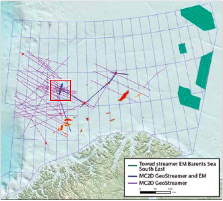
Using a towed streamer EM system makes it possible to use the same data to determine resistivity on a scale of a few hundred kilometres, and at the scale of the reservoir.

As part of the practical interpretation of CSEM data, the definition of anomalous zones of resistivity is one step in the overall workflow to determine the origin of high resistivity regions. However, the subsurface resistivity can vary by several orders of magnitude due to both lithology and fluid effects. In complex geological settings such as the Barents Sea the variation of resistivity that is possible means that it is important that we are able to determine the main regional factors controlling the variation of subsurface resistivity. Being able to define the background trend in, for example, electrical resistivity and anisotropy, is crucial in the robust interpretation of the subsurface and definition of areas considered anomalous. In essence we wish to be able to determine the subsurface resistivity at both the regional and reservoir scale.

Large and small scale resistivity

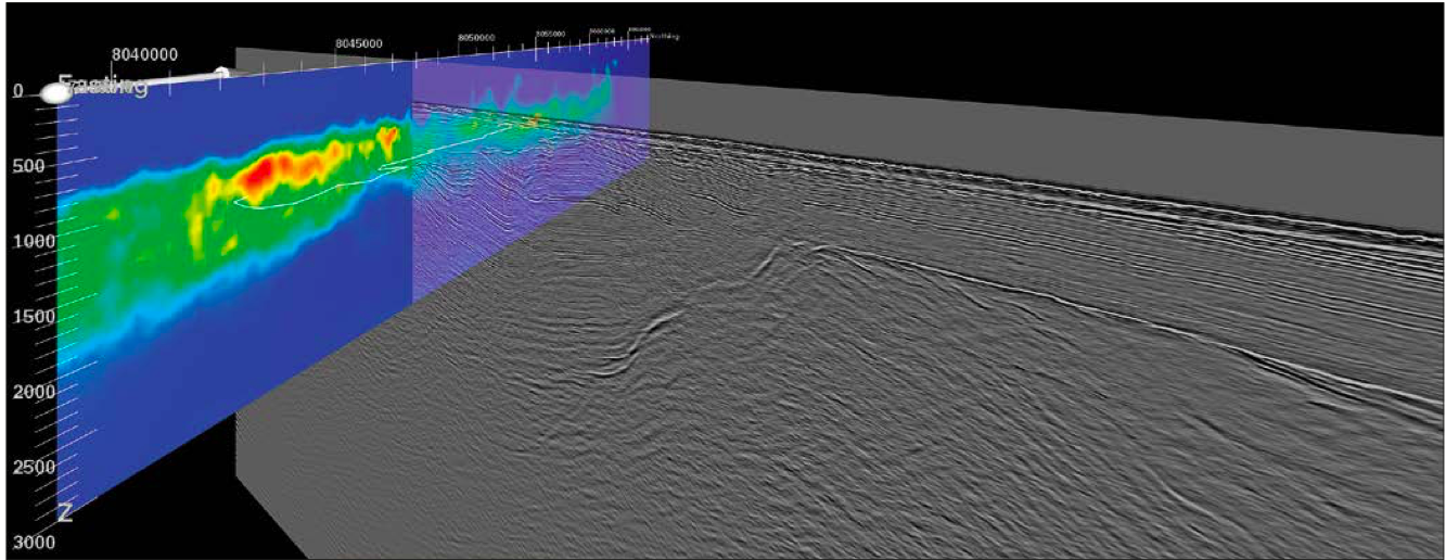
The fold-out figure on the previous page demonstrates the large scale of resistivity determination that is
now possible given that CSEM acquisition has been integrated with acquisition of broadband dual-sensor seismic data. The resistivity along the survey profile has been determined using unconstrained anisotropic 2.5D inversion, and is overlain on the full stack broadband dual-sensor data that was acquired at the same time. The horizontal component of resistivity is shown, and this is taken to represent the bulk background resistivity.

In the western part of the survey line the distinctive Bjørnøyrenna fault block terraces leading into the Bjørnoya Basin can be seen, while east of the Loppa High is the Bjarmeland Platform. The Loppa High is clearly one of the major units of resistivity on this survey line. In addition, a distinct structural difference in resistivity is observed – east of the Loppa High is generally more resistive than west of it. Each end of the profile indicates moderately resistive tertiary sediments: at the extreme western edge of the profile the increase in resistivity appears to be associated with an obvious gas-cloud zone.

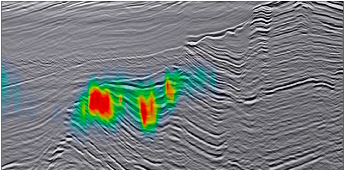
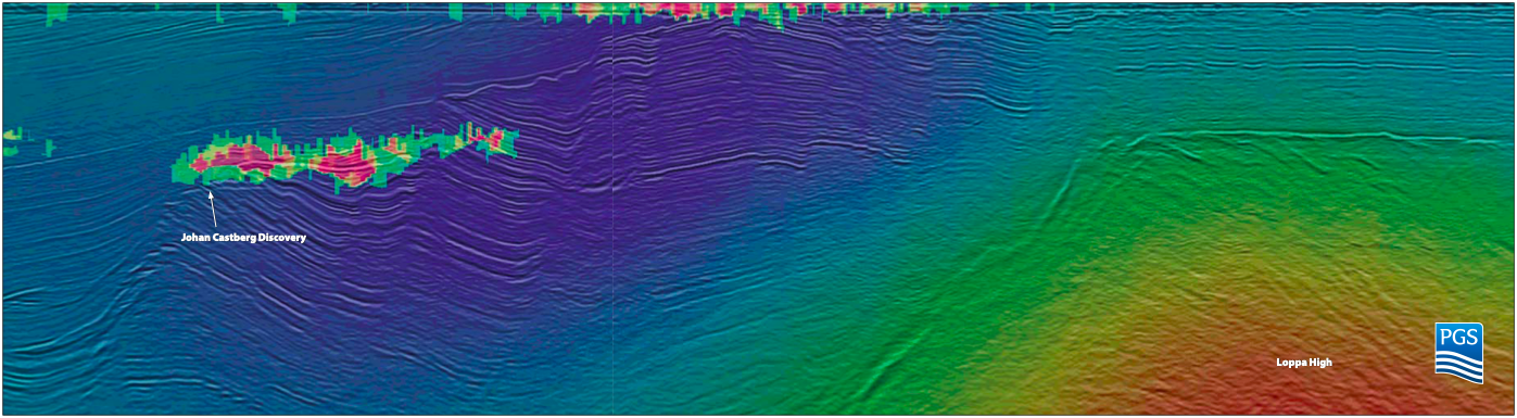
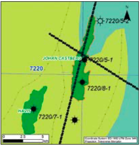
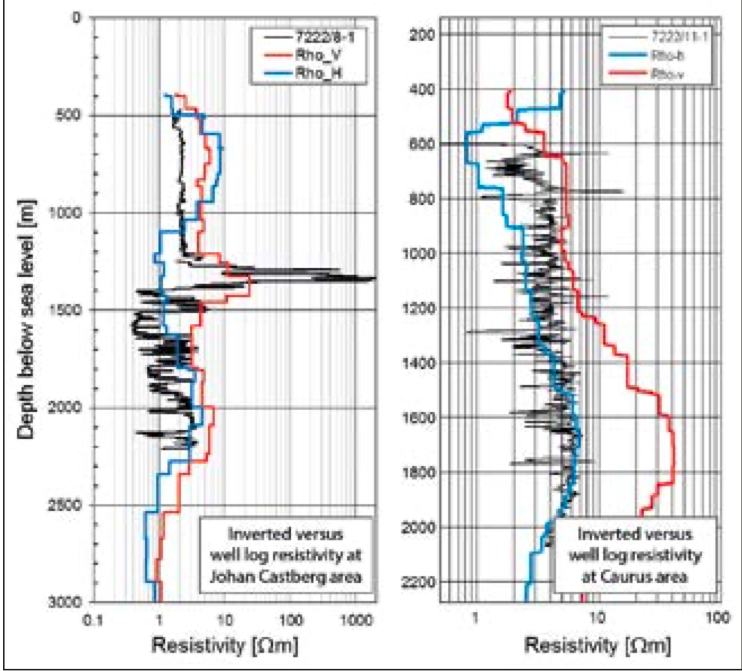
However, defining the background resistivity is only one piece of the puzzle – we also need to determine the resistivity at the reservoir scale. Shown below overlain on the seismic is the electrical anisotropy (ratio of vertical to horizontal resistivity) in the vicinity of the Johan Castberg discovery, determined using unconstrained inversion along a 20 km profile traversing Johan Castberg. The survey line crosses the short axis of the field (about 1.5 km wide) over the surface location of the 7220/5-1 appraisal well completed in 2012. There is a strong correspondence between high electrical anisotropy determined from inversion, and the Johan Castberg discovery. The strongest apparent anisotropy is restricted to the precise lateral location of the field, and is remarkably well registered in depth given that we have used unconstrained inversion. At the appraisal well location the top reservoir level is 1,276m below mean sea level; the oil water contact is at 1,395m and the apparent anisotropy anomaly is between 1,200 and 1,500m. Clearly, towed streamer EM data can be used to determine resistivity on a scale that ranges from about some tens of metres to 200 km.

Spatial data density

PGS’ towed streamer EM system allows for dense data sampling along the survey line and along the streamer cable itself. A typical transmitted electric current sequence from the source has a duration of 120s – representing a ‘shot’. With a towing speed of 4 knots, the system will move about 250m during this time. The acquired potential differences in the 72 electrode pairs in the streamer are deconvolved with the electric current sequence for every shot, which means that the resulting frequency responses of

the earth are estimated every 250m. The electrode pairs are evenly spread along the 8km streamer, which gives an average offset separation of about 100m. This is the highest spatial data density in the current version of the towed streamer EM system.  Are there any advantages to this data density compared to a more sparse acquisition? In particular, what happens with the subsurface resistivity image estimated from inversion when the frequency responses are decimated and are only obtained every 1,500m along a survey line? This is illustrated for a relatively simple resistivity structure in the following modelling example.

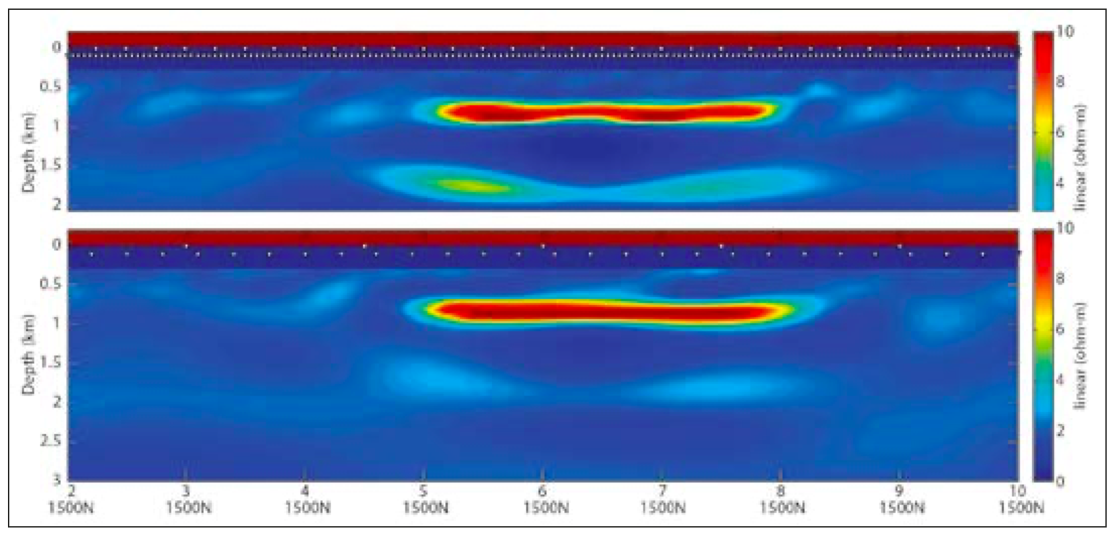
Consider a half space of an anisotropic background sediment with two high resistive anomalies. The subsurface model is located below a 300m layer of seawater of constant resistivity. An electric current source is towed 10m below the sea surface along a 21 km long survey line, with a streamer cable at a depth of 100m and with receiving electrode pairs every 100m. A 120s long source sequence is transmitted at every shot. The resulting frequency responses are then calculated at the frequencies of 0.1, 0.3, 0.5, 0.7 and 0.9 Hz for every offset and shot point.

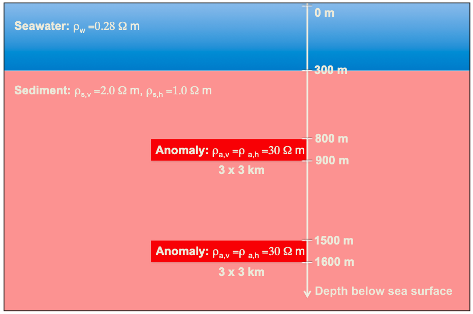
This synthetic data set is inverted using a 2.5D finite element inversion code called MARE2DEM with the vertical resistivity result shown in the top figure below. It can be seen that the top anomaly has been recovered rather well with a resistivity of 8–10 Ωm, whereas the lower anomaly is less well recovered but still visible. The horizontal extent of the top anomaly matches the model in the figure above very well, with an accuracy of 100m. The accuracy of the thickness is poorer since an unconstrained inversion was used, only preserving the product of anomaly thickness and resistivity value. In this case the recovered thickness is therefore roughly three times the true thickness, hence, a resistivity of about 10 Ωm.

The 2.5D inversion is now run with a spatially decimated data set where the shot and offset separations are 1,500m and 300m, respectively. The result is shown in the second figure below, where it can be seen that the lower anomaly has now almost disappeared. The top anomaly is still well recovered to within the same accuracy as with the denser data set.

The denser spatial sampling which can be achieved with a towed streamer EM system is demonstrated to be advant- ageous for a higher and more accurate vertical resolution of the subsurface and potentially allows the detection of deeper anomalies that would otherwise be missed.