“What is time then? If nobody asks me, I know; but if I were desirous to explain it to one that should ask me, plainly I do not know.”
Augustin, 332–430.
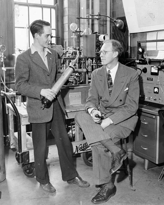
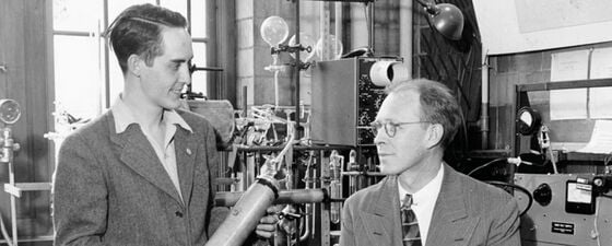
Figure 1: In 1946 Willard F. Libby (right), proposed an innovative method for dating organic materials by measuring their content of carbon-14, a newly discovered radioactive isotope of carbon. Known as radiocarbon dating, this method provides objective age estimates for carbon-based objects that originated from living organisms. Source: University of Chicago Photographic Archive, apf1-03868, Special Collections Research Center, University of Chicago Library.
We know that the atmospheric content of CO₂ has increased by 30% since 1958. It is much harder to measure and know where the extra CO₂ ends up after being emitted to the atmosphere. The nuclear bomb tests performed by the USA and the Soviet Union in the period from 1950 to 1962 led to a significant increase in radioactive carbon (14C) in the atmosphere. The radiocarbon dating laboratory in Trondheim initiated a large data acquisition effort in the 1960s aimed at monitoring the changes in radiocarbon that lasted until 1995. In this article we revisit this unique dataset and discuss briefly why this is of importance to our understanding of how CO₂ is circulating between the atmosphere, biosphere and the oceans.
The Trondheim Radiocarbon Dating Laboratory
The radioactive carbon isotope 14C disintegrates by emitting electrons (beta-decay). This process is slow, and it takes approximately 5,700 years before 50% of a given population of 14C atoms disintegrates, making it perfect for radiocarbon dating within a time range up to 50,000 years.
In the early 1950s a laboratory for 14C-dating was built in Trondheim at the Norwegian University of Science and Technology (NTNU) using solid carbon as the source. After several years, they could not show any positive results using this technique, so in 1955 professors Sverre Westin, Harald Wergeland and Reidar Nydal (Figure 3) decided to build a new laboratory based on CO₂ instead of carbon. This decision was based on a general recommendation from the radiocarbon dating conference that was held in Cambridge in July 1955. The professors in Trondheim asked for continued support from the Norwegian Research Council, and got a one year extension of the contract, and a strict message that if there were still no results within that time, the support from the council would end. The first sample that was tested in the new lab was a piece of wood from Caligula’s ship, which sank on Lake Nemi in Italy approximately 1,900 years ago. The size of the ship, designed as a luxury boat sailing on this small lake in Italy, was 70 × 20m. Caligula was Roman emperor from 12 to 41 CE, so in 1956 the age of the ship was probably around 1,925 years old (Figure 2). In the laboratory, Nydal and Sigmond estimated the age of the ship to be approximately 2,000 years, a result that secured continued support from the Norwegian Research Council.
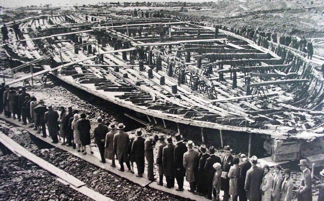
Figure 2: Italians viewing emperor Caligula’s ship (Prima Nave), which was found in 1932. As early radioactive dating techniques proved, the ship sank more than 1,900 years ago.
One of the first archaeological tasks for the laboratory was to determine the age of a monument built using timber, known as Raknehaugen, in Ullensaker in Norway that was formed as a huge cone, 95m wide and 15m high. The wood samples were determined to date from 540 +/– 50 years (CE).
In 1961 professor Anatol Heintz contacted the laboratory and asked them to determine the age of several mammoths from Siberia, who it was thought had fallen into ice rifts and died approximately 5,000 years ago. Several samples from various mammoths were analysed. Only one of the samples gave an age younger than the last ice age (11,450 years +/– 250 years), while six other specimens were dated as older than 30,000 years. Later, several mammoth samples were discovered in Norway, all of which were determined to be older than 40,000 years.
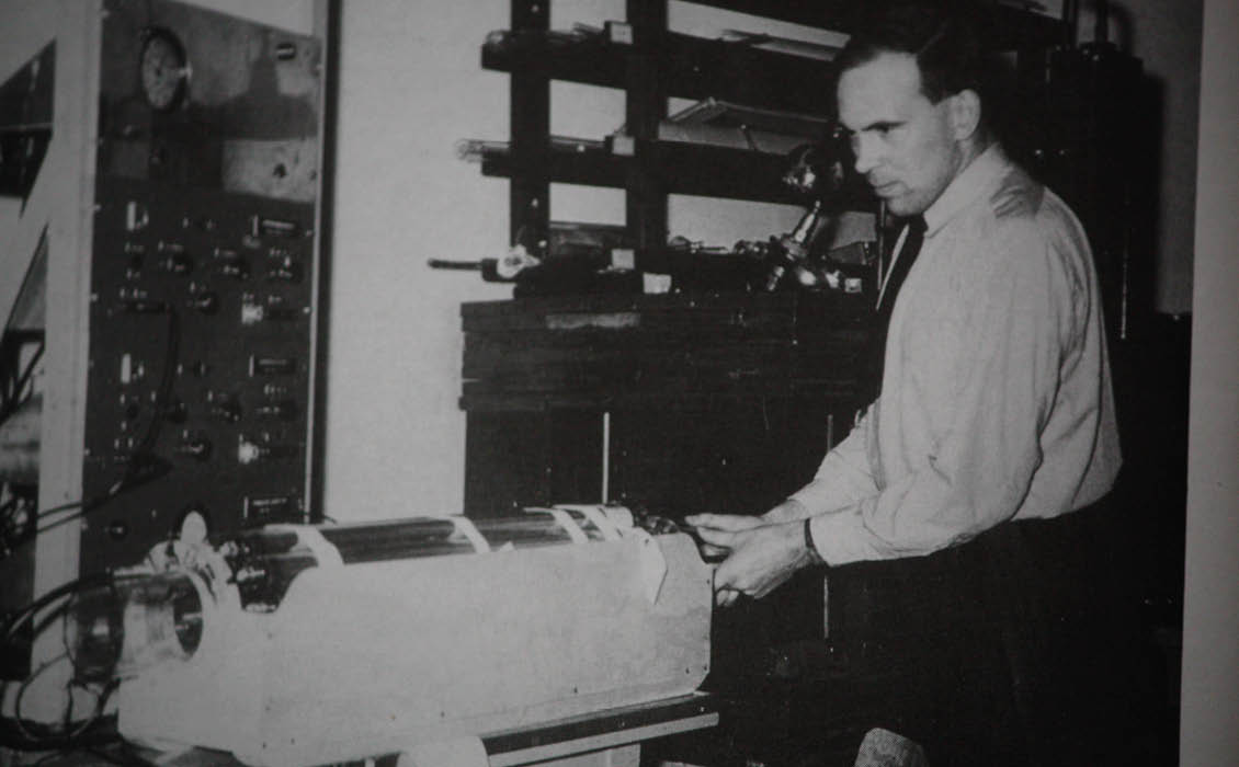
Figure 3: Reidar Nydal in the laboratory in 1955, testing Libby’s method for radiocarbon dating. Fortiden i søkelyset : 14C datering gjennom 25 år.
Background Radiation and Sample Contamination
It was evident from the beginning that the natural background radiation influenced the accuracy of the radiocarbon dating method significantly, especially for samples that were over 20,000 years old. Early in 1959 the typical background radiation for the laboratory in Trondheim was 10 events per minute. By improving the counters (electronics) as well as the surrounding screening (lead and steel) it was possible to lower the background radiation to approximately 0.5 events per minute. Similar laboratories in Bern and Seattle opted for locating the laboratory 50m below ground, to reduce the background radiation. When one of the Trondheim counters was tested in the subsurface laboratory in Bern it showed a rate of 0.3 pulses per minute. It was decided that the construction cost related to building a new underground laboratory in order to decrease the background radiation from 0.5 to 0.3 was not feasible.
Most of the samples are fairly easy to prepare and produce CO₂ from. A sample made of wood is burned while oxygen is added in a closed system, and liquid nitrogen is used to freeze the resulting CO₂ so it can be transported into the counter chamber. If the sample is a shell, the CO₂ can be released by adding acid. It is very important that the CO₂ gas is clean, because when organic material is burned or turned into CO₂, other gases like sulphur dioxide, chlorine gases and excess oxygen might capture some of the beta-radiation originating from a decaying 14C atom. Radon is another gas that will disturb a clean measurement. Fortunately, the radioactive radon gas has a short decay time, with a half-life of 3.8 days. This effect is simply solved by storing the CO₂ for approximately a month prior to the measurement.
Radiocarbon from Nuclear Tests
In 1962 the leader of the laboratory, Reidar Nydal, initiated a campaign to measure the increased 14C-levels in the atmosphere resulting from the nuclear bomb tests performed by the USA (from 1950–1959) and the Soviet Union (1961–1962). A treaty was signed 5 August, 1963, and both countries stopped testing these large hydrogen bombs. However, China, France and the UK did not sign this treaty and these countries continued to undertake nuclear bomb tests in the period from 1964 to 1974.
Nydal’s great acquisition plan covered stations all over the world, including Norway, Madagascar, Ethiopia, Senegal, Chad and the Canary Islands. In addition, he established an agreement with the Norwegian shipping enterprises Wilhelmsen and Fred Olsen whereby crew on board the ships were trained to produce CO₂ from seawater samples. To get a sufficient amount of CO₂, typically 200 litres of seawater was needed. One of the authors of this article (ML) was a laboratory assistant for the academic year 1977–1978. He found it a pleasure to work with Reidar Nydal, and exciting to prepare and analyse the seawater samples that had been gathered by the ships.
In 1996 Reidar Nydal and Knut Løvseth organised all the data that has been acquired relating to 14C measurements in a database. Figure 4a shows measurements of 14C (increase above normal) for the period between 1963 and 1993. In the first couple of years we observe a seasonal oscillation that is less pronounced later. These oscillations are observed in Norway, being close to Novaja Zemlja where the Soviet Union detonated bombs equivalent to a strength of 337 Mtonnes. The distance from Novaja Zemlja to Fruholmen in Northern Norway (where one of the stations was located) is approximately 1,000 km.
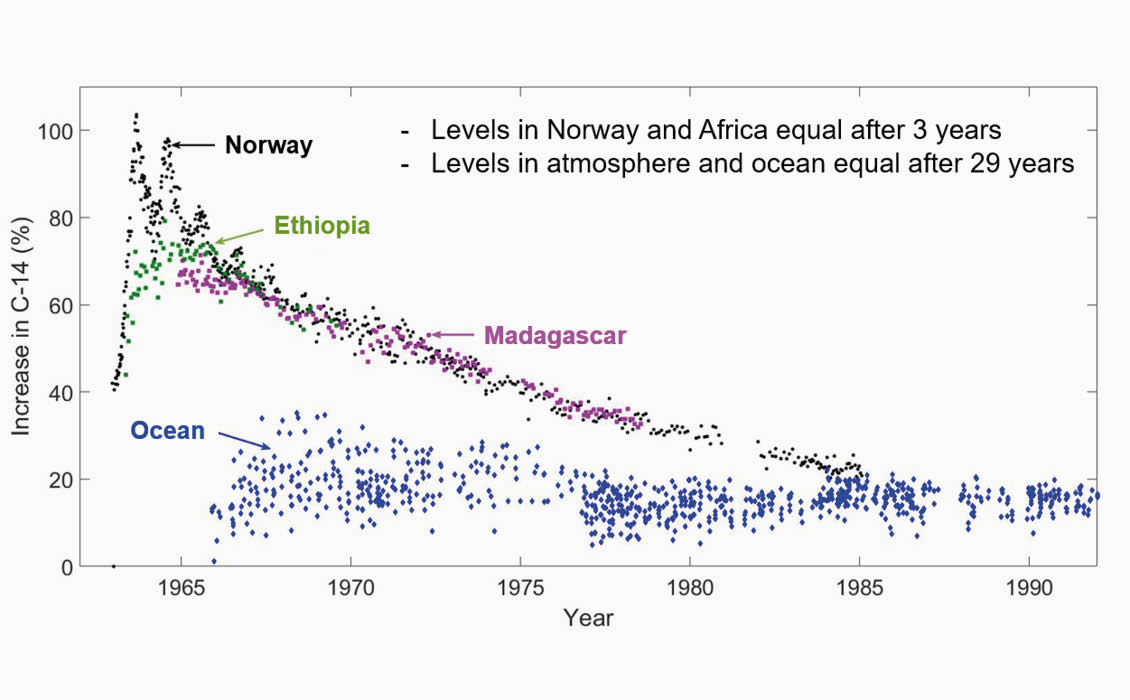
Figure 4a: Measurements of increased 14C in the atmosphere and the ocean. Data source: Nydal and Løvseth, 1996.
We notice that the radiocarbon levels in Norway and Africa are equal in 1966–1967, three years after the treaty was signed. The figure also includes all the seawater samples that were acquired between 1966 and 1993. These samples cover a huge part of the oceans including the Atlantic and Pacific. Ship routes including passages through the Panama and Suez channels are included in this dataset. All seawater samples were taken close to the surface, so there are no depth variations in these data. After 30 years we observe that the relative increase in radiocarbon is equal for the atmosphere and the ocean.
Radiocarbon Absorbed in Humans
Nydal acquired blood samples from two people in Trondheim from 1963 to 1978. He also analysed hair samples from one person within the same period. The blood and hair samples show similar behaviour, and 2–3 years after 1963 the levels in the human body seem to follow the atmospheric levels, as shown in Figure 4b.
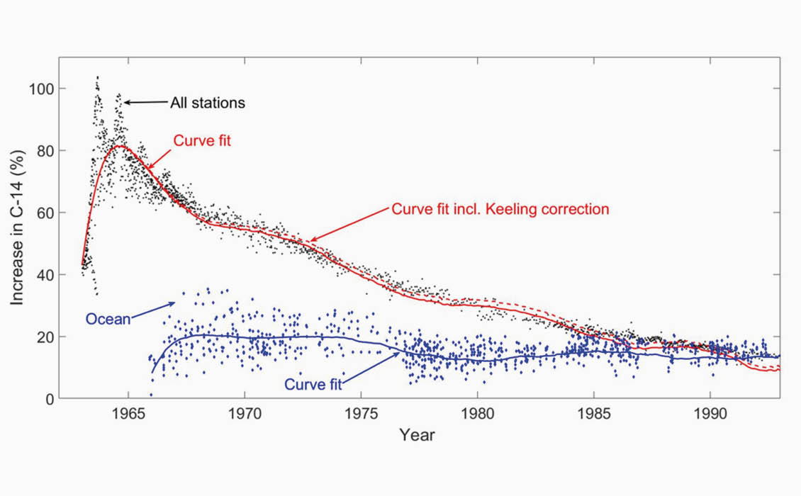
Figure 4b: Variation in 14C above normal between 1963 and 1985, measured in the atmosphere in Norway and in human blood and hair samples from Norwegian citizens.
Nydal made a simple box model including the stratosphere (10–30 km), the troposphere (0–10 km), the biosphere and the ocean. He concluded that radioactive carbon emitted by bombs that were detonated in 1961 and 1962 had an average lifetime in the stratosphere of two years, followed by a one-year lifetime in the troposphere. The average life of a carbon atom in the atmosphere that enters into the ocean is approximately seven years. How the CO₂ mixes with deeper layers in the ocean cannot be studied using these data.
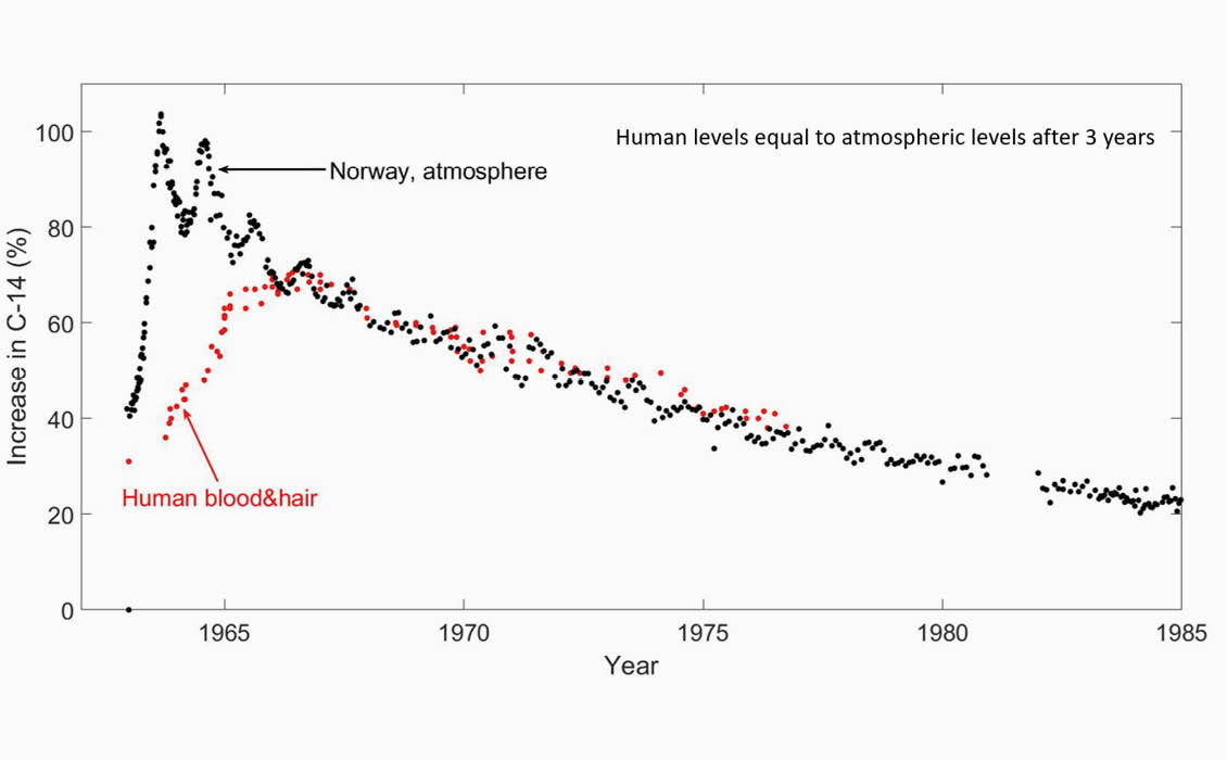
Figure 4c: Variation in 14C above normal for all land stations and ocean samples.
All Land and Ocean Samples If all 14 land stations are included as well as all the ocean data, we clearly see in Figure 4c that the radiocarbon levels approach a 15% increase above normal after approximately 30 years. A simple curve fit to the data is also shown in this figure, and we observe that the curves for the atmosphere and the ocean cross each other around 1992. In the period from 1963 to 1993 the CO₂ level in the atmosphere rose from 315 ppm to 356 ppm (a 13% increase). The CO₂ emitted by fossil fuels is neutral with respect to radiocarbon content. The red dashed line shows the curve fit assuming that the total amount of CO₂ had been constant at 315 ppm over the whole period.
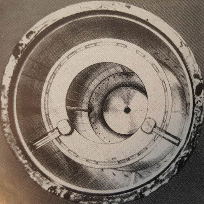
Figure 5: The first 14C- counter device used by the radiocarbon dating laboratory in Trondheim. The inner cylinder is filled with CO₂ gas and the 14C atoms are counted in an electric field between the outer lattice and the centre cord (not visible on the photo). Fortiden i søkelyset: 14C datering gjennom 25 år.
Reference
Fortiden i søkelyset : 14C datering gjennom 25 år. https://cdiac.ess-dive.lbl.gov/epubs/ndp/ndp057/ndp057.html#
Further Reading in the ‘Recent Advances in Climate Change Research’ Series
Recent Advances in Climate Change Research: Part I – Blackbody Radiation and Milankovic Cycles
Martin Landrø and Lasse Amundsen, NTNU / Bivrost Geo
Geoscience will probably play an important role in mitigating carbon dioxide emissions. In part one of this series, we discuss some history and physics behind the topic of climate change including the concepts behind blackbody radiation and Millankovic Cycles.
This article appeared in Vol. 16, No. 2 – 2019
Recent Advances in Climate Change Research: Part II – Arrhenius and Blackbody Radiation
Martin Landrø and Lasse Amundsen, NTNU / Bivrost Geo
In Part II we look at Arrhenius’ seminal 1896 paper and see how it relates to blackbody radiation and absorption of infrared radiation by the atmosphere, taking a closer look at his model of the greenhouse effect.
This article appeared in Vol. 16, No. 3 – 2019
Recent Advances in Climate Change Research: Part III – A Simple Greenhouse Model
Martin Landrø and Lasse Amundsen, NTNU/Bivrost Geo
What would the temperature of Earth be without the atmosphere? By using simple physical models for solar irradiation and the Stefan-Boltzmans law for blackbody radiation, we can estimate average temperatures with and without atmosphere.
This article appeared in Vol. 16, No. 4 – 2019
Recent Advances in Climate Change Research: Part IV – Challenges and Practical Issues of Carbon Capture & Storage
Martin Landrø, Lasse Amundsen and Philip Ringrose
The basic idea behind CCS (Carbon Capture and Storage) is simple, but what are the main challenges and practical issues preventing a more global adoption of this method?
This article appeared in Vol. 16, No. 5 – 2019
Recent Advances in Climate Change Research: Part V – Underground Storage of Carbon Dioxide
Eva K. Halland, Norwegian Petroleum Directorate. Series Editors: Martin Landrø and Lasse Amundsen, NTU/Bivrost Geo
By building on knowledge from the petroleum industry and experience of over 23 years of storing CO₂ in deep geological formations, we can make a new value chain and a business model for carbon capture and storage (CCS) in the North Sea Basin.
This article appeared in Vol. 16, No. 6 – 2019
Recent Advances in Climate Change Research: Part VI – More on the Simple Greenhouse Model
Lasse Amundsen and Martin Landrø, NTNU/Bivrost Geo
We continue the discussion of the simple greenhouse model introduced in Part III.
This article appeared in Vol. 17, No. 1 – 2020
Recent Advances in Climate Change Research: Part VII – Arrhenius’ Greenhouse Rule for Carbon Dioxide
Lasse Amundsen and Martin Landrø, NTNU/Bivrost Geo
Here, we investigate the relationship between radiative forcing (heat warming) of carbon dioxide and its concentration in the atmosphere to better understand climate feedback and sensitivity.
This article appeared in Vol. 17, No. 2 – 2020
Recent Advances in Climate Change Research: Part VIII – How Carbon Dioxide Absorbs Earth’s IR Radiation
Lasse Amundsen and Martin Landrø, NTNU/Bivrost Geo
Skydive with us into the quantum world and find out how carbon dioxide molecules absorb thermal IR radiation.
This article appeared in Vol. 17, No. 3 – 2020
Recent Advances in Climate Change Research: Part IX – How Carbon Dioxide Emits IR Photons
Lasse Amundsen* and Martin Landrø, NTNU/Bivrost Geo
Skydive with us into the quantum world, where we provide to those unafraid of molecular energy transfer an answer to the question: what happens to Earth’s radiated infrared (IR) photons after they are absorbed by IR active CO₂ molecules in the lower atmosphere?
This article appeared in Vol. 17, No. 4 – 2020