How AVO has been and continues to be an essential tool in de-risking the world’s high-impact exploration wells
People tend to say that a good geologist has seen many rocks. But does the same apply to geophysicists? Is a geophysicist more knowledgeable when he or she has seen more seismic data? I’m not aware of that same principle being used. What I do know, however, is that the two people I spoke to for this article have seen a lot of seismic activity from all over the world.
Henk Kombrink
Henry Pettingill, who is a geologist by training, became the head of the Rose DHI Consortium after having been a member for eighteen years. Geophysicist Rocky Roden has been a principal in the DHI Consortium for 25 years. Together with their colleagues Mike Forrest and Roger Holeywell, they have seen an unparalleled number of exploration programmes and discussed the subsequent drilling results that have all been thoroughly assessed for DHI’s. This happens at regular meetings of the consortium members from over 30 companies, during which the work done on de-risking prospects is discussed privately, such that learnings can be shared.
Rocky and Henry tap into this experience when informing me about the basic principles of AVO, followed by a discussion on the most common pitfalls, how prospect risking is done in practice, and what the future of AVO-driven exploration entails. But let’s start with the basics first.
The 1950’S and beyond
Our understanding of DHI’s has evolved from Gassman’s fluid replacement modelling in 1951, to the recognition of the relationship of bright spots and hydrocarbons, and subsequently to AVO changes with offset due to gas observed by Ostrander in 1984.
Nowadays, AVO is a standard tool in the exploration toolkit. That is not a coincidence, as the geological success rate of AVO-supported wells has been significantly higher than that of wells drilled without.
“It is also good to mention that AVO is only one of the geophysical methodologies that fall under the Direct Hydrocarbon Indicator umbrella. Some people think that every DHI has a strong AVO effect, but DHI’s from stacked data, such as flat spots and edge effects are often more diagnostic. AVO is just one of the tools in the DHI toolbox,” says Rocky.
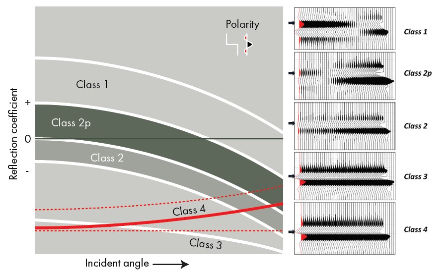
Figure 1. Classification scheme for the five different AVO Classes, showing how amplitudes change with offset at the top gas sands. Source: modified from Rutherford and Williams (1989); Castagna and Swan (1997); and Ross and Kinman (1995).
Figure 1 shows the classification scheme on how amplitudes change with offset at the top of gas sands. Nowadays, typically five classes are distinguished, but when Steven Rutherford and Robert Williams came up with the first proper classification of AVO classes in 1989, only Classes 1, 2 and 3 were defined. “There was quite some discussion on how to name or number them,” says Rocky. “We had Steven Rutherford present at our DHI consortium a few years ago, and he recalled the story of the discussion they had whether to call them 1, 2, 3; A, B, C or X, Y, Z. Only at the last minute, they went for 1, 2, and 3.”
That was fortunate, as in subsequent years, Class 4 was added to the mix through the work of John Castagna and Herbert Swan in 1997. John Castagna has made numerous contributions to the Consortium through the years. In addition, a subdivision of Class 2 into two sub-classes was introduced through the work of Chris Ross and Daniel Kinman in 1995, where Class 2P includes a phase reversal with offset, whereas Class 2 does not.
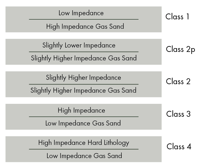
Figure 2. Note that it is the relative impedance contrast between the overlying seal and the gas sand below that ultimately determines the AVO Class. Source: DHI Consortium.
Careful classification
“The five Classes provide a framework for interpreting AVO, but what really determines the AVO Class for prospects is the following,” says Rocky. “Look at the relative acoustic impedance contrast between hydrocarbon reservoirs and the overlying lithology (shale) in Figure 2; in some cases, a gas sand is low impedance, in others it is high. Basically, all combinations between seal and reservoir are possible, and therefore we have to be careful in assigning an AVO class before we have done an integration with other geological data.”
“An example is a well in the Barents Sea we had the privilege to review. We had a 20 % porosity reservoir, typically a Class 2 AVO, but it also had a source rock sitting on top of it. And because that source rock had such low impedance, it looked like a Class 1 AVO. There are several places around the world where we can observe this, and it shows that it’s not only the reservoir that determines the Class, but the combination with what sits above it.”
AVO EXAMPLES
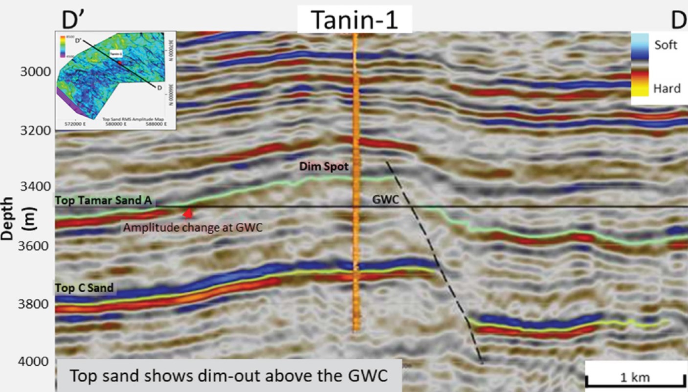
Class 1: The Tanin gas discovery in the Eastern Mediterranean (Egypt) is a great example of a Class 1 AVO response, with amplitudes dimming at top reservoir level when moving from the water-wet to gas-bearing in the Tamar Sand A sand. A Class 1 AVO usually occurs in consolidated reservoirs, where porosity tends to be reduced at deeper levels. Because of the compacted nature of Class 1 sands, and the impedance difference between the sands and seals becoming smaller, the number of Class 1 AVO prospects in the DHI Consortium database of 415 wells is very limited.
Figure 3. A Class 1 AVO response, showing a dimming of the top reservoir reflector at the Tanin gas discovery, offshore Egypt. Source: El-Ata et al. (2023),Sci Rep 13, 8897.
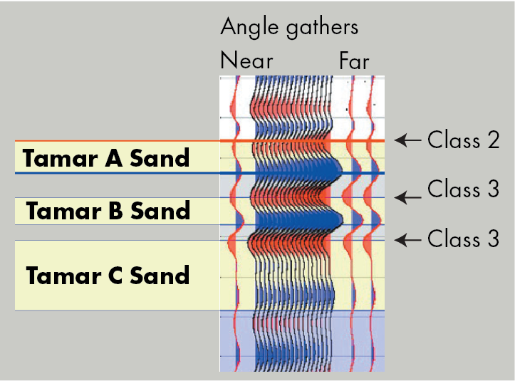
Class 2: AVO’s tend to develop in slightly less compacted and consolidated sands than the Class 1 examples. The difference between a Class 2 and 2P AVO response is that the latter shows a polarity reversal whilst the former doesn’t. Both AVO classes experience a negative gradient (slope) as the offset increases. An example of a Class 2 AVO response can be seen in the Tamar gas discovery offshore Israel, where a series of Miocene sands proved to be gas-bearing. As can be seen in Figure 4, the top sand (A) shows a Class 3 response from slightly negative to a more negative response with offset.
Figure 4. The Tamar gas discovery offshore Israel shows both Class 2 as well as Class 3 AVO responses, as shown here. Adapted from: Needham et al. (2017), AAPG Memoir 113.
Class 3: Because of the strongly negative response Class 3 AVO shows at the whole range of offsets, this class is also known as the Bright Spot AVO. With increasing offset, the amplitudes become even slightly more negative than they already are at near-offset. The Tamar B and C sands are examples of Class 3 AVO responses (Figure 4).
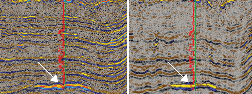
Figure 5. Near-angle stacked seismic data (left) and Far-angle stacked seismic data for the Hoover field, Gulf of Mexico, showing a gentle dimming from Near to Far. Source: Inyang (2009), Master Thesis University of Houston.
Class 4: Many Class 4 AVO’s occur in unconsolidated sands, similar to Class 3 AVO’s. But as Figure 1 already shows, the change of amplitude over offset is small, which means that the identification of a Class 4 AVO can be tricky. The example shown here corresponds with that observation, with a Class 4 from Hoover Field, Gulf of Mexico, where the Far-angle stack shows a slightly more subtle amplitude response than the Near-angle stack.
AVO pitfalls
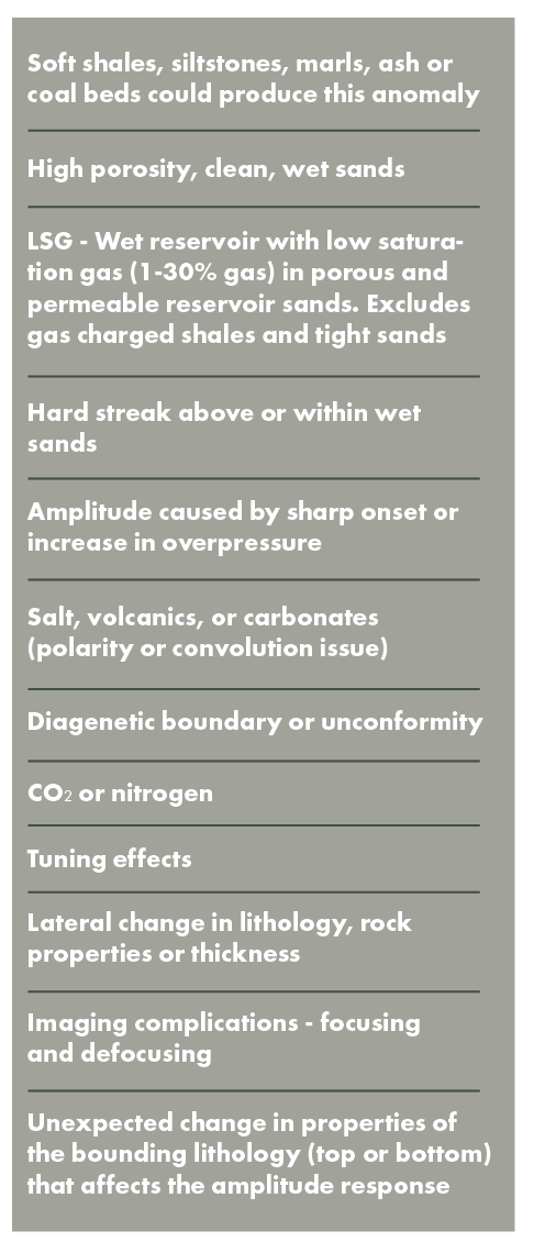
“For me,” says Henry, “the very reason why we have pitfalls in the first place is because of the non-unique nature of geophysical solutions and therefore AVO. Multiple scenarios can explain the same geophysical expression. That’s why we always walk through a list of potential pitfalls, asking ourselves what might be other explanations to explain the amplitude response we see.” This list of potential pitfalls is briefly summarised in Figure 6.
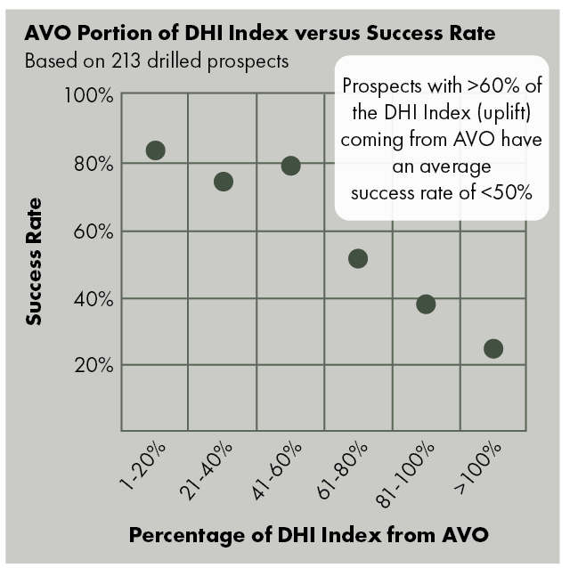
“If the contribution to the DHI-uplifted chance of success associated with AVO gets too high, compared to the other DHI characteristics, we see a decrease in prospect success rates,” adds Rocky. “Uncalibrated AVO is the main reason for this. Most high-quality DHI prospects have numerous DHI characteristics, and a dominantly AVO-driven prospect therefore increases the risks.” The drop in success rate is illustrated in Figure 7; when the AVO part of the DHI Index is more than 60 %, the chance of success is greatly reduced.
Below are a few of the more important pitfalls interpreters have to be mindful of.
AVO tuning
“If you look at a gather,” starts Rocky, “and it is not spectrally balanced, you often encounter Normal Moveout Out stretch as you get to the far offsets. This subsequently causes a lower frequency on the far offsets.”
“So, if you have an uncalibrated thick wet sand, and it starts to tune right at the associated frequency, typically at the mid to far offsets, it blossoms because of the tuning effect. In turn, this looks like a hydrocarbon effect. It’s a difficult thing to get your head around unless you do a lot of modelling. However, it is very resolvable; all you have to do is spectrally balance your gathers, such that you don’t have any frequency changes across the gathers. Some companies will do this routinely, some of them will not.”
“We know at least two to three cases in the DHI Consortium where AVO tuning effects produced inaccurate interpretations that led to failed drilling attempts. There are probably more in our database, but detailed modelling was not performed on these dry holes to confirm AVO tuning,” concludes Rocky.
Figure 6. Checklist of most common pitfalls for interpreting DHI’s and associated AVO effects. Can these pitfalls cause amplitude and AVO features that can be misinterpreted to be DHI’s? Note: LSG does produce a hydrocarbon effect, but usually indicative of a seal or trap failure.
Ash beds and other soft non-reservoir lithologies
About 20 % of failed DHIs are caused by non-reservoir lithologies – soft shales, marls, silts and ash. “We have seen the latter in the Gulf of Mexico, but also in the West of Shetlands,” says Henry, “and it has been a thing that has hit me at regular intervals throughout my career.”
“The first time was with Shell when we drilled Natasha in the Gulf of Mexico in the early 1980’s, where we thought we had a good downdip conformance with structure, but we drilled a Pleistocene ash turbidite instead. It was the first time we hit such an ash bed in the area, but many more have been drilled since, in many levels ranging from Lower Miocene to Pleistocene.”
“Twenty years later, when I was with Noble, we were going to drill the Stone’s River prospect in the Mississippi Canyon, far away from Natasha. What happened? The beautiful Class 2 AVO turned out to be yet another sand containing 30 % ash.”
“And that was not all. Twenty years later, at a company’s office in Houston, we were discussing a prospect that had some sub-salt issues, and we were going down the road of discussing everything that could have gone wrong with this prospect, except what? A forty-year career, and being burnt at 20-year increments by the same pitfalls,” Henry laughs.
Wet sands
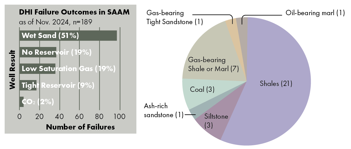
“Half of the number of the dry holes in our database are wet sands,” says Henry, “and most of those, when looking back, had a decent AVO response.” See Figure 8 for an overview of the share of other factors contributing to drilling dry holes.
“You can get a response from a wet sand,” continues Rocky, “but if you don’t know anything else, and it is a Class 3 AVO with a small gradient in a frontier area without any calibration points, it will be hard to make a differentiation between a gas or water-bearing sand. Sometimes you are just in the margin of error bars. That’s why we always try to look at as many characteristics as we can to find further evidence of hydrocarbons.”
“Once we drilled four thick wet sands in a row with Noble,” says Henry, “which obviously raised some eyebrows in the company. So, I called Rocky in as a consultant at the time to have a more detailed look at it. We had a discovery called Isabela, with another prospect on the flank of the same four-way structure. It looked all good, with an element of stratigraphic trapping that we were confident about, and a similar AVO response as the Isabela find. However, this prospect came in dry. It was Rocky who then identified that the rock properties of the topseal changed from one well to the other, and this is what caused the AVO response in the downflank prospect, rather than a gas-filled sand. It opened my eyes, as it was such a good example of non-uniqueness and simply how the rocks determine it all.”
“Mind you, a few years later in Australia, something similar happened but, in this case, with a more positive outcome. It was the Enfield area, where the discovered field had a nice bright amplitude, but the nearby prospect that they were looking at didn’t have nearly as good an AVO response as the discovery, despite the geology being similar. So the first thing that popped into my mind after seeing the variable top-bounding shales in the wells was, maybe there is a bounding lithology change. And sure enough, there was, and it was a discovery despite having a weaker AVO signature.”
Changing data quality
The DHI consortium keeps an impressive database (The Seismic Amplitude Analysis Module, SAAM) of 415 wells that have all been assessed and risked in the same way. Not only for AVO, but also for other DHI Characteristics such as brights spots, flat spots, downdip conformance and phase reversal amongst others. A geological chance of success is also assessed to ultimately determine the final calibrated chance of geological success for the prospect.
Figure 7. The AVO portion of the overall DHI Index should not be too high, as an analysis based on 213 drillled prospects has shown. A significant drop in success rate takes place when prospects rely on AVO for more than 60% of the DHI Index. Source: DHI Consortium.
The database is a powerful tool to review, rank and evaluate the world’s most important exploration wells, but in order to properly compare them, one must be mindful of the change in data quality that has taken place over the years.
“The gathers and overall data quality we see today are superior to what we saw at the start of our consortium 25 years ago. During the first five years, we hardly saw any gathers at all, because they were too expensive to generate,” says Rocky. “If you don’t correct for data quality somehow, you can have a good prospect with bad data having a poor ranking compared to a bad prospect with good quality data. That’s why we introduced the data quality score, which aims to account for variations in data quality, especially when risking prospects of different seismic vintages.”
“But at the same time, even with the advancements of better data, a lot of prospects today can be more complicated,” says Rocky. “Things don’t stand out anymore as they used to. We have got sub-salt prospects, stratigraphic prospects, all sorts of geological challenges that we were not looking for 25 years ago.” “And to that I can add that gathers are still not perfect,” says Henry. “Things can look good, but that doesn’t necessarily mean they are correct.”
Henry then pulls up a prospect drilled in the Gulf of Mexico not too long ago. The overall DHI Index of the prospect came out at 22 %, with the AVO part being 13 %. That’s on the edge of being too AVO driven,” explains Henry. “We want a prospect to have a healthy mix of DHI factors.”
Where are we going?
Kenny Goh, a geophysicist who recently commented on one of our LinkedIn posts, wrote: “ExxonMobil geophysicists mentioned to me that they do not believe that AVO responses at 2,200 m below mudline and 2,400 m water depth in Jubilee are correct or real.”
So, I asked Rocky what his take on it is. “As rocks get buried deeper and deeper,” Rocky explains, “they will become harder and as such, the impedance contrasts between them will gradually decrease. So the presence of hydrocarbons may not produce an anomaly. That’s where the Class 1 AVO response comes in, where the reservoir is very compacted and as a result, the fluid effect on the AVO response is very small. For that reason, we have only seven Class 1 prospects in our database.”
“So when it comes to defining the DHI floor these days, as the depth limit of direct hydrocarbon indicators is sometimes called, it really depends on the basin you are in,” explains Rocky.
Figure 8. Wet sands form 51% of the cases where a DHI was incorrectly interpreted as a hydrocarbon indication (left graph). Looking at the failures where a lack of reservoir formed the root cause, it is shales that are most frequently found in those cases (right). Data based on analysis by the DHI Consortium.
“Subsalt makes that even more complicated. Up to a few years ago, there was a general consensus that you couldn’t believe DHIs subsalt,” says Rocky. “Maybe you could map a structure, but surely you wouldn’t believe the amplitudes. But it is thanks to new technology, primarily FWI and the application of ocean bottom nodes, that we are slowly getting more confidence in the quality of sub-salt seismic imaging for amplitudes. Maybe, in a few years time, we will be just as confident risking prospects sub-salt as we are post-salt.”
AVO IN CARBONATES – AN INDIRECT HYDROCARBON INDICATOR
“You’re opening up a whole different subtopic here,” says Henry when I ask him about the role of DHIs and AVO in carbonates. “However, we always get asked about it during presentations, and we will present on the topic at the upcoming IMAGE Conference in Houston, so it is definitely a hot topic.”
At the basis of it all, the AVO classification for sands simply does not apply to carbonates. The complex pore structure of carbonates tends to cause a scatter of velocities, complicating the seismic quantification of the parameters. In addition, carbonates often have a higher velocity heterogeneity and anisotropy than sands, which does not facilitate interpretation either.
“Against that backdrop,” Henry adds, “when people say that they found oil in Paleozoic carbonates based on AVO, as that is what happened with quite some Midcontinent discoveries in the past, I tend to believe that the AVO effect was due to enhanced porosity development in the carbonates rather than the fluid fill itself. So in these cases, AVO should probably be seen as an indirect hydrocarbon indicator in carbonates at best, and no universal AVO classification scheme can simply be applied to carbonates at the moment.”
“It is also telling that we only have five carbonate DHI examples in our database that consists of 415 wells.”
“Computing power is still the challenge to make incremental improvements to the seismic though, especially sub-salt” adds Rocky. “FWI is an optimisation process that is computationally expensive, and processing for sub-salt imaging routinely takes months and months to complete.”
“But quantum computing is maybe coming to the rescue. Last year alone, I saw four papers being published on the use of quantum computing in geophysics. The use of quantum computing for seismic imaging and modelling is in its infancy, but the largest technology companies and governments are committing billions of dollars to resolve the issues to make it work.”
“To me, it is extremely exciting to follow these developments,” concludes Rocky, “as it has the potential to produce phenomenal results once the quantum computing code is cracked. Imagine a future where elastic FWI is routine and DHI analysis, including AVO evaluation, incorporates data far superior to anything we have today.”