Seismic inversion is essentially a very simple procedure. In a seismic inversion the original reflectivity data, as typically recorded routinely, is converted from an interface property (i.e. a reflection) to a rock property known as impedance, which itself is the multiplication of sonic velocity and bulk density. In a conventional seismic reflectivity section the strong amplitudes are associated with the boundaries between geological formations, such as the top reservoir. This type of data is most suited to structural interpretation. In an inverted dataset the amplitudes are now describing the internal rock properties, such as lithology type, porosity or the fluid type in the rocks (brine or hydrocarbons). Inverted data is ideal for stratigraphic interpretation and reservoir characterization.
Figure 1 compares a conventional seismic reflectivity section with the simplest form of inversion, known as a relative impedance, which is directly estimated from the seismic with no model inputs and so is a robust and reliable seismic property. This particular example uses a method developed by BP known as colored inversion, which is the best type of relative impedance currently available.
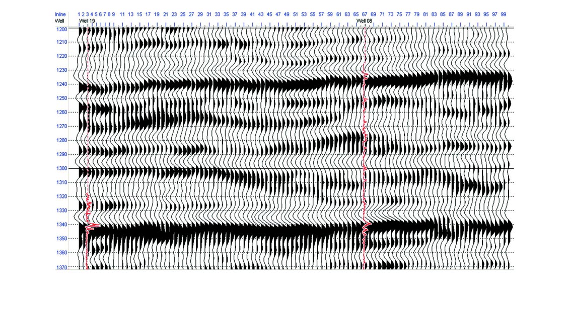
Figure 1: Conventional seismic reflection data compared with colored impedance data. The sand intervals are shown as the blue/purple colors.
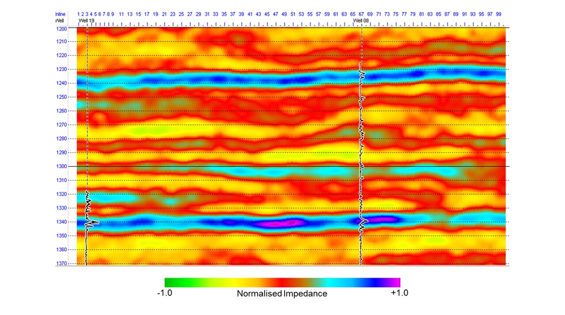
Figure 1: Conventional seismic reflection data compared with colored impedance data. The sand intervals are shown as the blue/purple colors.
One feature of a relative inversion such as colored inversion is that the data is trendless. For example, because porosity decreases with depth we would expect impedance to increase with depth as the geological formations become harder and faster with compaction. However, a relative impedance seismic volume is trendless both vertically and laterally, because trends are by definition very low frequency features of the data and seismic does not record very low frequencies. Therefore an important rule to understand about relative impedance is that it does not inform us about trends.
Deterministic Inversion
In a deterministic inversion the missing low frequency is introduced to the inversion, thus giving the appearance of trends. However, in effect, the missing low frequency trend is simply modeled and added to the relative impedance result, so a deterministic inversion is really just a modeled trend plus a relative impedance. The result can look like it has strong vertical and lateral trends present but great care must be taken when interpreting this data because these trends are not from seismic reflections but are from a smoothly interpreted model.
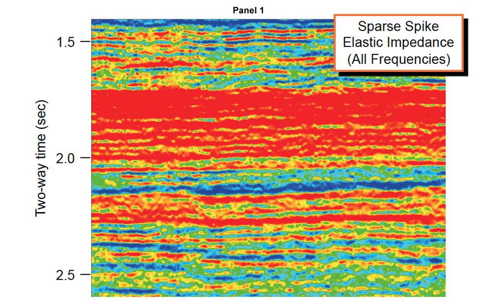
Figure 2: Panel 1 is the result of a deterministic inversion, while Panel 2 shows the low frequency model used to create the deterministic inversion. Panel 3 shows the deterministic inversion after the model has been removed and Panel 4 shows the relative inversion only, of the original seismic. Note that the deterministic inversion without model (Panel 3) is essentially identical to the relative inversion (Panel 4).
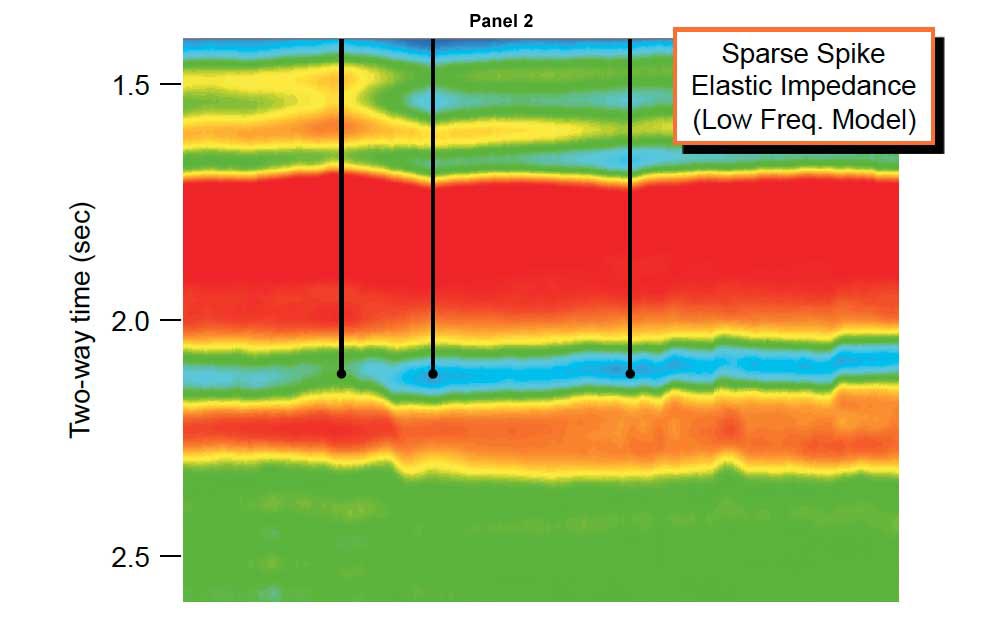
Figure 2: Panel 1 is the result of a deterministic inversion, while Panel 2 shows the low frequency model used to create the deterministic inversion. Panel 3 shows the deterministic inversion after the model has been removed and Panel 4 shows the relative inversion only, of the original seismic. Note that the deterministic inversion without model (Panel 3) is essentially identical to the relative inversion (Panel 4).

Figure 2: Panel 1 is the result of a deterministic inversion, while Panel 2 shows the low frequency model used to create the deterministic inversion. Panel 3 shows the deterministic inversion after the model has been removed and Panel 4 shows the relative inversion only, of the original seismic. Note that the deterministic inversion without model (Panel 3) is essentially identical to the relative inversion (Panel 4).
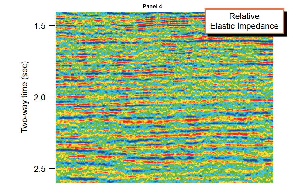
Figure 2: Panel 1 is the result of a deterministic inversion, while Panel 2 shows the low frequency model used to create the deterministic inversion. Panel 3 shows the deterministic inversion after the model has been removed and Panel 4 shows the relative inversion only, of the original seismic. Note that the deterministic inversion without model (Panel 3) is essentially identical to the relative inversion (Panel 4).
A demonstration of the influence of the model is shown in Figure 2. You will note that the deterministic inversion without model is essentially identical to the relative inversion, hence the general statement that deterministic inversion = relative inversion + model.
Although great care must be taken in interpreting trends from deterministic inversion, if the model is carefully constructed and if the seismic response is comprised of strong amplitudes at the target reservoir then a deterministic inversion may be used for mapping and lateral prediction. Some examples of mapping porosity in this way are illustrated in Figure 3.

Figure 3: Stratigraphic slices through a deterministic inversion result calibrated to porosity. Good porosity areas shown in red.
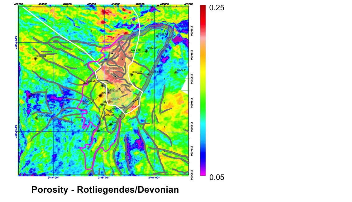
Figure 3: Stratigraphic slices through a deterministic inversion result calibrated to porosity. Good porosity areas shown in red.
Simultaneous Inversion
Pre-stack seismic data contains additional information about the rock properties of the earth and these can be inverted for, using several different methods. A common one is simultaneous pre-stack inversion, a form of seismic inversion which inverts for several rock property parameters simultaneously using the pre-stack gather (or partial stacking of this data, such as angle stacks). Usually simultaneous pre-stack inversion is a deterministic inversion, so as noted above great care must be taken with the results to ensure that what is interpreted is seismic data and not the model. After pre-stack simultaneous inversion it is often safer to filter the model out of the results using a high pass filter.
If sufficient angle ranges in the seismic gathers have been successfully processed then it may be possible to invert seismic data for three properties, sometimes called three-term inversion. This requires good quality seismic including processed angles above 40° and is not always possible. More commonly and very routinely seismic is inverted using a two-term approach, which is quite reliable and possible with most seismic reflection datasets where pre-stack data is available. This method of inversion gives two output rock properties, typically P-wave (sonic) impedance and S-wave impedance. These can be combined to create two further properties known as lambda-rho (λρ) and mu-rho (μρ). In general P-wave impedance (IP) and λρ properties inform us about pore space effects such as porosity and hydrocarbons (presence or saturation). S-wave impedance (SI) and μρ inform us about lithology, with the effects of the pore space and fluids removed. By comparing a rock property anomaly between each type of output it is possible to get a better understanding as to whether the anomaly may be caused by porosity/saturation changes or by lithology changes.
If three-term inversion is possible then the result will be sonic, shear and density parameters. These are usually in the form of P-wave (sonic) impedance, S-wave impedance and bulk density. The additional bulk density term is quite difficult to invert for from seismic as its contribution to the overall seismic amplitude is small and only present on large angles (greater than 40°).
Seismic inversion results are very often calibrated to some other rock property. The calibration can be after the inversion, for example to convert a seismic property to estimate porosity. An example is shown in Figure 3 of a stratigraphic horizon slice from a deterministic seismic inversion, calibrated to porosity. Two different stratigraphic levels are shown, with red corresponding to high porosity. Although this is a good quality inversion and is controlled by many wells, we should note it is a deterministic inversion and so care should be taken not to over-interpret trends which may be coming from the imposed model and not the seismic data. One way to guard against this problem is to request the model to be supplied with the final deterministic inversion and check that the trends interpreted are not artefacts from the model building.
EEI Inversion
It is also possible to perform a type of calibration before inversion. This is where the pre-stack data is combined to create new seismic properties which are most closely related to properties such as petrophysical quantities like porosity or shale volume. A robust and natural way to achieve this is to use a method called Extended Elastic impedance or EEI, again invented by BP. An extended elastic impedance uses the angle gather information (the same information required by a pre-stack simultaneous inversion) and projects the data across new angles using standard AVO intercept and gradient analysis. The new angles required as output are chosen to correspond to rock or petrophysical quantities of interest, such as porosity or shale volume, usually by analyzing well log data. EEI uses a special angle term called Chi (χ) which can have a continuous projected range from -90º to +90º.
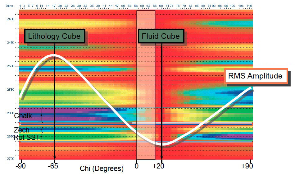 Figure 4: A modeled example of EEI impedance as a function of Chi angle using well logs. The vertical axis is time and the color display is of the relative impedance as a function of the Chi angle (horizontal axis). Note how the amplitude strength varies with Chi angle. Zero Chi angle corresponds to P-wave (sonic) impedance and around -45° corresponds to S-wave impedance, as does mu-rho. Lambda-rho is typically about +30°.A modeled example using well logs is shown in Figure 4. The beauty of EEI is that it gives a continuous range of possibilities from -90º to +90º, not just properties that correspond to geophysical parameters such as the ones described above. this makes it possible to select a seismic property volume for a Chi angle that corresponds to a petrophysical quantity such as shale volume, making the result much more interpreter friendly. Alternatively, two characteristic angles can be found for seismic datasets, one of which corresponds to the Chi angle at which the largest amplitudes occur and is referred to as the ‘lithology cube’ and one at the Chi angle associated with the minimum angles. This is often called the ‘fluid cube’, although a better description would be the ‘pore space cube’ as it is generally sensitive to both fluid types and porosity.
EEI results are often presented as relative or colored impedance, and can also be output as a deterministic inversion.
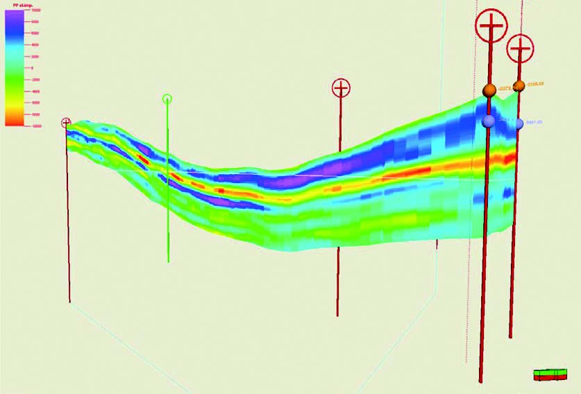
Figure 5: In the first panel a seismic colored-impedance property, derived from the process described in Figure 4, is displayed in the reservoir model cells. In the middle panel the shale volume property (Vshale or Vsh) has been simulated in the model using only the wells as inputs – note the detail in the layering. In the final panel the shale volume has been simulated in the model using the wells and the seismic impedance data in the first panel. Note how the good reservoir (not purple) is smooth and strongly connected. This is probably not realistic and arises because of the low resolution of the seismic impedance.
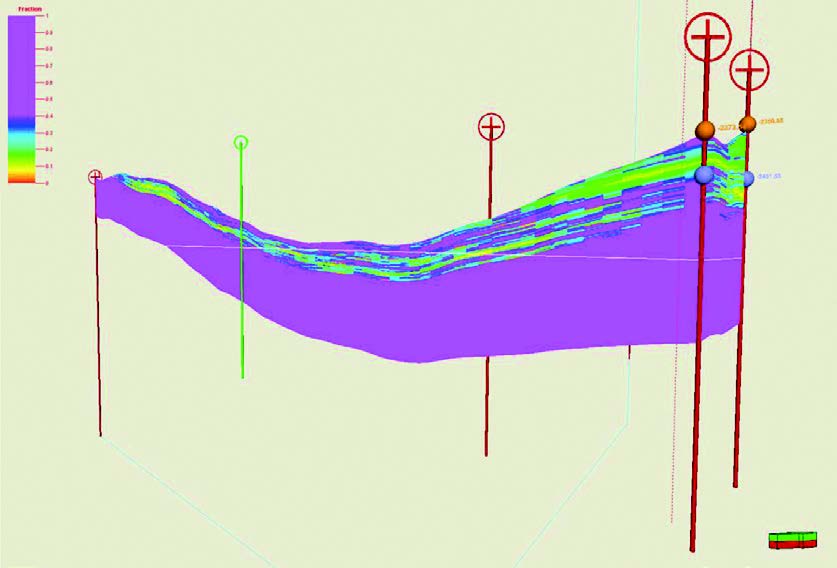
Figure 5: In the first panel a seismic colored-impedance property, derived from the process described in Figure 4, is displayed in the reservoir model cells. In the middle panel the shale volume property (Vshale or Vsh) has been simulated in the model using only the wells as inputs – note the detail in the layering. In the final panel the shale volume has been simulated in the model using the wells and the seismic impedance data in the first panel. Note how the good reservoir (not purple) is smooth and strongly connected. This is probably not realistic and arises because of the low resolution of the seismic impedance.
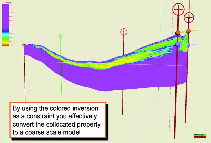
Figure 5: In the first panel a seismic colored-impedance property, derived from the process described in Figure 4, is displayed in the reservoir model cells. In the middle panel the shale volume property (Vshale or Vsh) has been simulated in the model using only the wells as inputs – note the detail in the layering. In the final panel the shale volume has been simulated in the model using the wells and the seismic impedance data in the first panel. Note how the good reservoir (not purple) is smooth and strongly connected. This is probably not realistic and arises because of the low resolution of the seismic impedance.
Inversion and Reservoir Modeling
Seismic inversion output is quite attractive for guiding the mapping of properties like facies distribution or porosity in reservoir modeling. However, great care should be taken in using inversion data in this way.
One problem is the effect of seismic ‘tuning’, where the amplitudes of the inversion respond not just to the rock properties but also to the thickness of the bed. if the thickness is close to the ‘tuning’ frequency of that particular seismic then the amplitude can appear much brighter than it really is, possibly causing thickness changes in the beds to be misinterpreted as rock property changes. this problem affects relative and colored inversion. It is sometimes claimed that deterministic inversion removes the effects of tuning, but in general this is not the case. Tuning effects must be removed before inversion data can be used in reservoir models.
A second problem with using seismic inversion data in reservoir modeling is the large difference in vertical resolution between the model and the seismic impedance. A model typically has a vertical cell resolution of 1m, but seismic inversion is more typically a vertical resolution of 20m. Constraining the reservoir property at 1m scale to a seismic property at 20m scale is incorrect and can lead to poor models which can give misleading fluid flow characteristics. An example of this is shown in Figure 5.
An additional problem is the model in a deterministic inversion. If this model is left in the seismic property used to map properties in a reservoir model, then we are in danger of making our reservoir model follow the trends of another model we have created! This is clearly a serious problem and so the model part should be removed from a deterministic inversion.
Stochastic Inversion
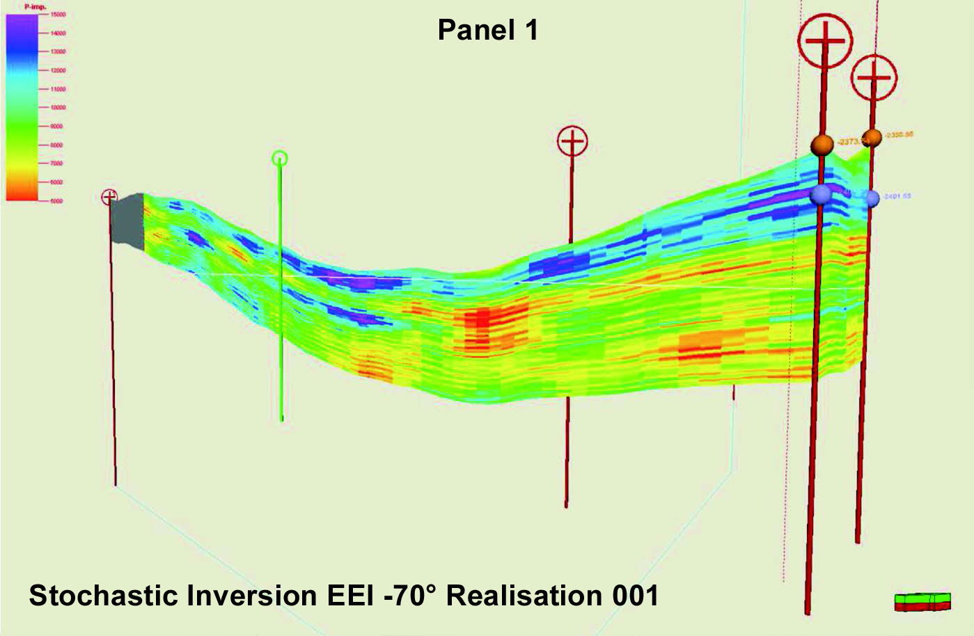
Figure 6: Panels 1-3 are different geostatistical realizations of impedance generated from a stochastic inversion. The differences between these realizations highlights the uncertainty in a seismic inversion that is modeled in a stochastic inversion. Note also how much more detailed and realistic they are than the smooth colored impedance result shown in the final panel of Figure 5 above. Panels 4-6 are shale volume simulations in the reservoir model, each constrained by the stochastic inversion realization as indicated in the label.

Figure 6: Panels 1-3 are different geostatistical realizations of impedance generated from a stochastic inversion. The differences between these realizations highlights the uncertainty in a seismic inversion that is modeled in a stochastic inversion. Note also how much more detailed and realistic they are than the smooth colored impedance result shown in the final panel of Figure 5 above. Panels 4-6 are shale volume simulations in the reservoir model, each constrained by the stochastic inversion realization as indicated in the label.
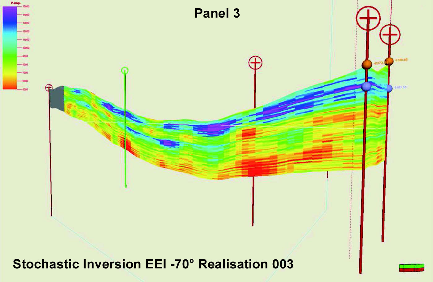
Figure 6: Panels 1-3 are different geostatistical realizations of impedance generated from a stochastic inversion. The differences between these realizations highlights the uncertainty in a seismic inversion that is modeled in a stochastic inversion. Note also how much more detailed and realistic they are than the smooth colored impedance result shown in the final panel of Figure 5 above. Panels 4-6 are shale volume simulations in the reservoir model, each constrained by the stochastic inversion realization as indicated in the label.
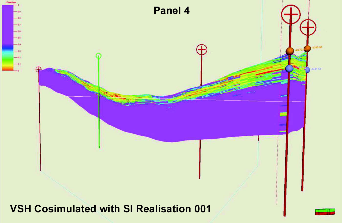
Figure 6: Panels 1-3 are different geostatistical realizations of impedance generated from a stochastic inversion. The differences between these realizations highlights the uncertainty in a seismic inversion that is modeled in a stochastic inversion. Note also how much more detailed and realistic they are than the smooth colored impedance result shown in the final panel of Figure 5 above. Panels 4-6 are shale volume simulations in the reservoir model, each constrained by the stochastic inversion realization as indicated in the label.

Figure 6: Panels 1-3 are different geostatistical realizations of impedance generated from a stochastic inversion. The differences between these realizations highlights the uncertainty in a seismic inversion that is modeled in a stochastic inversion. Note also how much more detailed and realistic they are than the smooth colored impedance result shown in the final panel of Figure 5 above. Panels 4-6 are shale volume simulations in the reservoir model, each constrained by the stochastic inversion realization as indicated in the label.

Figure 6: Panels 1-3 are different geostatistical realizations of impedance generated from a stochastic inversion. The differences between these realizations highlights the uncertainty in a seismic inversion that is modeled in a stochastic inversion. Note also how much more detailed and realistic they are than the smooth colored impedance result shown in the final panel of Figure 5 above. Panels 4-6 are shale volume simulations in the reservoir model, each constrained by the stochastic inversion realization as indicated in the label.
 Stochastic inversion (or geostatistical inversion) is the technique of simulating possible rock property models using the seismic. This has many technical advantages for use in reservoir modeling and uncertainty analysis: it removes tuning effects, it models the uncertainty and it can be computed at fine scale; but these advantages must be weighed against its higher cost and the large data quantities that must be managed. A comparison of a stochastic inversion used in a reservoir model is shown in Figure 6.
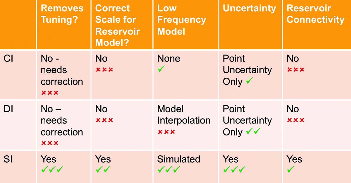
There are many flavors and variants of seismic inversion and only the most general ones have been compared here. As a quick guide, the following table provides comparison showing the good features (green ticks) and the bad features (red crosses) of the various methods.