Middle Jurassic Broom sandstones from the Hudson field, UK Northern North Sea. Photography: Henk Kombrink.
Evaluating the uncertainty in a Saturation Height model
Uncertainty is present in everything we do with subsurface data, so trying to understand the impact of that uncertainty in our interpretations and models, both static and dynamic, is essential
Even the ‘ground truth’ of core data is uncertain when you really think about it. There is nothing better than a lump of rock to look at, touch, smell, or even lick (if you are so inclined) to provide some certainty about the rocks. Some data is very subjective, like facies description, but what about the hard data, the ‘facts’, that we calibrate our models to? Every core measurement, including depth, porosity, permeability and capillary pressure (Pc), has uncertainty, even cutting the core and recovering it to surface alters it from the in-situ condition. When you consider all the uncertainties in the data used to build a saturation height model, then it can feel like quantum mechanics, a bit fuzzy, and very often a lot fuzzy.
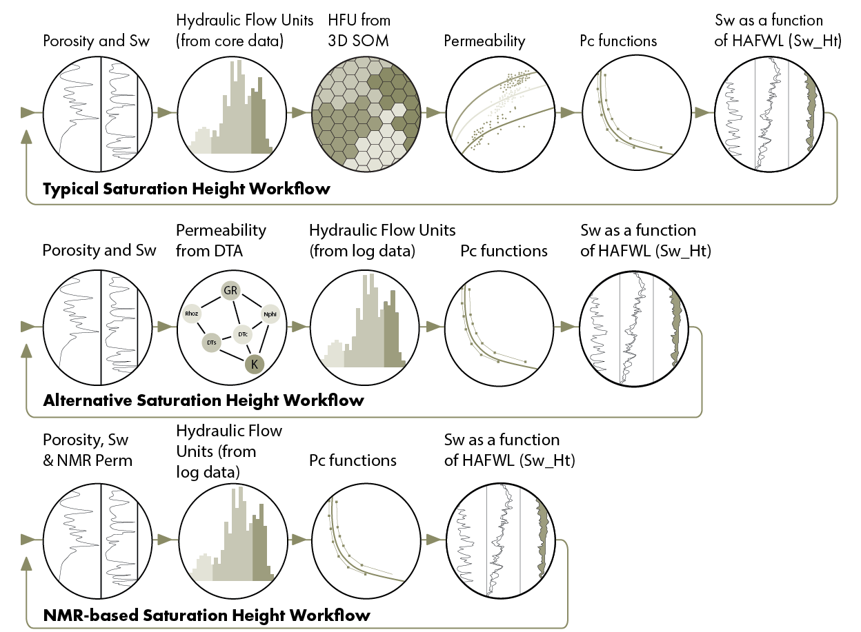
A typical workflow to develop a saturation height model makes use of a variety of data and interpretations, from log and core.
This may include the following steps:
- An interpretation of the logs to determine porosity and water saturation (Sw) in the wells
- An interpretation of the core data to determine the hydraulic flow units (HFUs)
- Extend the HFU model from core to the wells, with a predictive model using the log data, trained on the core derived HFUs, e.g. with a 3D Self Organising Map (SOM)
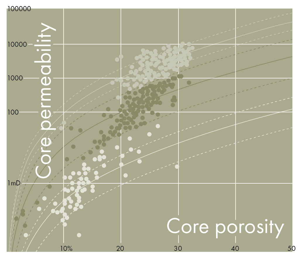
- Use the HFU por-perm relationships, with the porosity and predicted HFU, to determine permeability in the wells
- Fit functions to the core Pc data, for each HFU
- Apply those functions in the wells to determine water saturation from the model (Sw_Ht)
- Compare Sw_Ht to the Sw from step 1 and adjust the model to get the ‘best’ fit
This last step is where most of the hard work is, because every step could be adjusted or completely changed. It’s not just about the R2 in fitting the function to the Pc, it’s about everything. Is the log-derived porosity correct? What about the Sw? Have we identified the correct number of HFUs in the core? Do we have the right boundaries? Can we robustly predict the HFUs in the wells? This is a complex task, and why many petrophysicists and reservoir engineers often dedicate so much time to it.
There are many choices to be made at every step, such as which volumetric methodology to use and which predictive model to use, but even the number and order of these steps is a choice that depends on data availability and preference. One alternative approach is to use a predictive model for permeability instead of the HFU, e.g. using Domain Transfer Analysis (DTA), and then use that permeability with the porosity in the HFU model. That reduces the number of steps to 5.
Another alternative is to use NMR log permeability, removing the need for a predictive model and reducing the number of steps to 4.
These different workflows all contain uncertainty, so how do we decide on the ‘best’ model, the most fit-for-purpose model? We can, of course, just pick the workflow that gives the closest match to the log-derived Sw, but there are other aspects to consider, such as how this model will be implemented in the dynamic model.
If the permeability used in the model came from the HFU por-perm relationships, they can be applied directly in the dynamic model. This means that both static and dynamic models are consistent, using exactly the same relationships, removing a common source of uncertainty. If a predictive model was used for the permeability in the static model, you may get a better fit to Sw, and you have reduced the number of steps in the workflow, but that predictive model cannot be implemented in the dynamic model. Typically, a separate HFU por-perm model will be used for that, meaning there is a disconnect between the static and dynamic models, re-introducing uncertainty. Its swings and roundabouts.
Ideally, we would quantify the uncertainty in these models, to help decide which is the ‘best’, and this can be done with a Monte Carlo uncertainty analysis on the entire workflow. We cannot Monte Carlo all of the choices in the workflow, there are too many possibilities and it becomes an infinite problem, but we can run the numbers on the entire workflow, end-to-end. For example, in a Monte Carlo run, we can numerically quantify the uncertainties in the following steps:
- The inputs logs: Every log has a published tolerance, e.g. RHOB +/- 0.02 g/cc, so we can use that, and in a rugose borehole it will be even more uncertain
- The interpreted results: Every numeric parameter affecting every result, such as porosity, mineral volumes and Sw, has uncertainty, even those we may think we know, e.g. Rw. Did it come from produced water? Was it picked in a clean wet zone? Or based on an assumption?
- The HFUs: We consider the HFU model ‘fixed’, meaning the number of flow units and their boundaries, and the predictive model ‘fixed’, having been trained on the HFU data, but running the predictive model will yield varying distributions of HFUs across the wells as we are capturing the uncertainties in the inputs, whether they are logs or interpreted results
- The permeability: We can use the P10, P50 and P90 of the por-perm relationship for each HFU
- The Sw_Ht results: We consider the functions ‘fixed’, as Sw_Ht will change with changes in porosity and permeability, but we can also apply uncertainty to the FWL, GOC, fluid densities and IFT correction factors
By applying all these uncertainties together, in each Monte Carlo iteration, and running the entire workflow hundreds or thousands of times, each with slightly different parameters, we can quantify the impact of the different porosity, flow unit, permeability, and function on the final Sw_Ht. If we include a calculation of hydrocarbon-pore-feet (PhiSoH) for the interval in question, for each iteration, then the P10, P50 and P90 of the PhiSoH shows the overall uncertainty in the entire workflow. That way different workflows can be quantitively compared, rather than the subjective “I like that one as it looks better.”