In a recent Oilvoice article, well known industry figure David Bamford suggested a better term to describe what seismic interpreters do was ‘subsurface detectives’, rather than ‘explorers’. Just like police detectives solving a crime, interpreters collect lots of evidence, sift through it and analyse it before constructing their interpretations. However, working with angle stacks alone, subsurface detectives can’t tell if their evidence has been compromised or corrupted in some way. The real quality of the data is hidden behind the stacks and only inspection of the seismic gathers can give a true answer as to the reliability of the seismic evidence and, therefore, the robustness of the interpretations.
Working with limited information selected from the vast database of available evidence, subsurface detectives can easily miss vital clues and come to the wrong conclusions. Without accessing the whole data volume, they cannot confidently look for patterns, anomalies and inconsistences in the evidence and thereby understand the uncertainties and risks within; correctly assessing the probability of success.
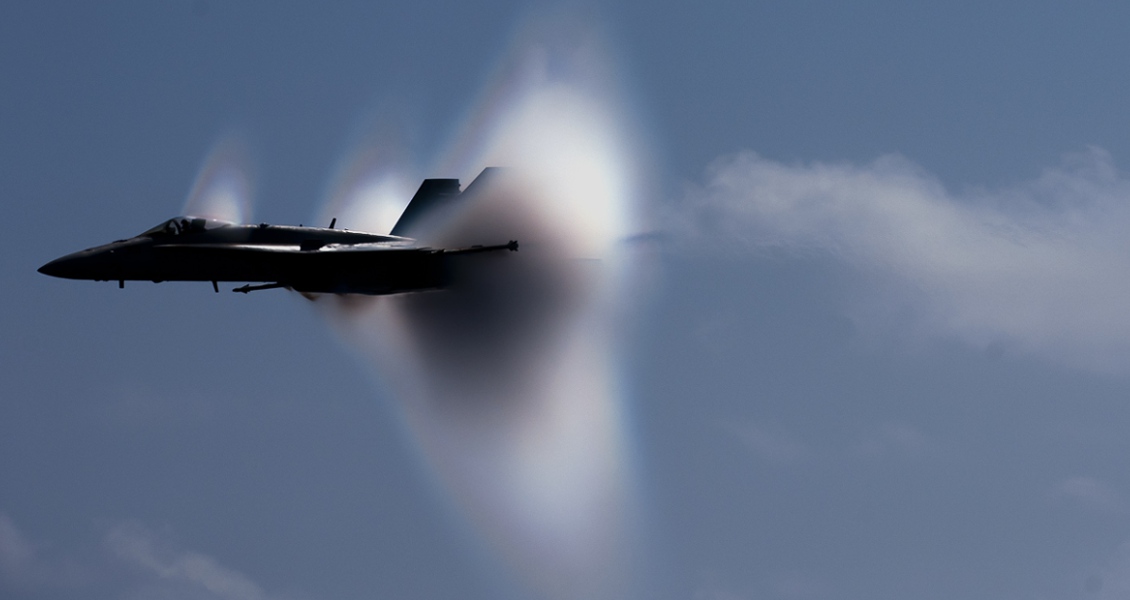
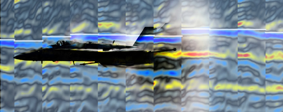
An F/A-18C Hornet breaks the sound barrier. The white halo formed by condensed water droplets is thought to result from an increase in air pressure around the aircraft at transonic speeds. (Source: U.S. Navy. Travis K. Mendoza. Wiki commons)
Like the ‘sound barrier’, which became a psychological as well as a physical barrier for pilots and aeroplanes – the ‘stack barrier’, marking the domain boundary between seismic processors and seismic interpreters, has somehow remained stubbornly in place, if not in the software we use, in our minds and our psyche! It sometimes seems we are too frightened that our interpretations, so carefully constructed flying through stack data, will not stand up to the shaking they receive as we cross the ‘stack barrier’ to mine the rich information available in the pre-stack data. For example, the more accurate fluid prediction, gained by using interactive AVO/AVA attributes directly from gathers, can help identify potential reservoirs and distinguish hydrocarbons from water.
And yet we have all seen the value of moving our interpretation focus down the processing sequence, from paper to colour graphics displays, from attribute sections to original seismic stacks, from post-stack processed seismic to raw stacks; so we should embrace the idea, get comfortable with handling gathers and enjoy the ride.
Computer hardware and software advances have allowed us to fully manipulate and visualise, all of our stacked seismic data volumes, to guide interpretation. Today’s multicore hardware and optimised parallel-processing seismic interpretation software now allow the same kind of manipulation and visualisation for pre-stack gather volumes – a breaking of the stack barrier for interpreters and an opening up of a ‘view-and-do’ stack and pre-stack combined interpretation world.
For example, discrete, single gathers can be placed inside a 3D scene alongside surfaces, faults, well bores etc and usually attached dynamically to a post-stack seismic section, made from stacking them. Figure 1 (below) shows two examples, displayed using OpendTect interpretation software from dGB.
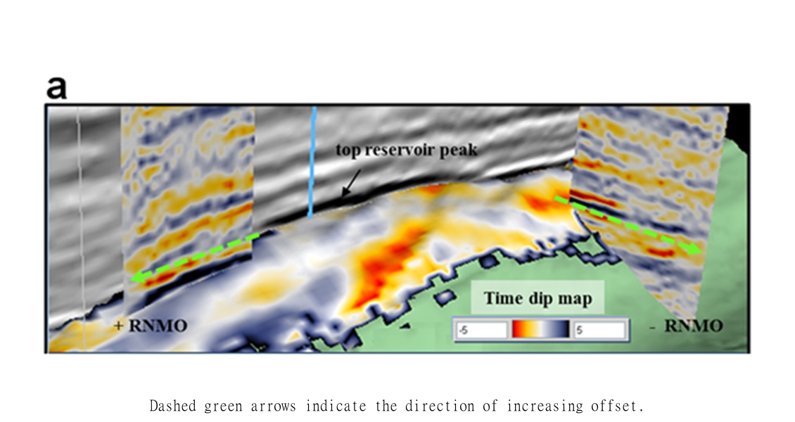
Figure 1a. 3D view of the top of a chalk reservoir. The time dip with offset map and the gathers, displayed in context with the rest of the field‘s data, allow the interpreter to investigate where any velocity differences may be coming from – such as channeling or fracturing parallel to structure, changing porosity and fluid content?
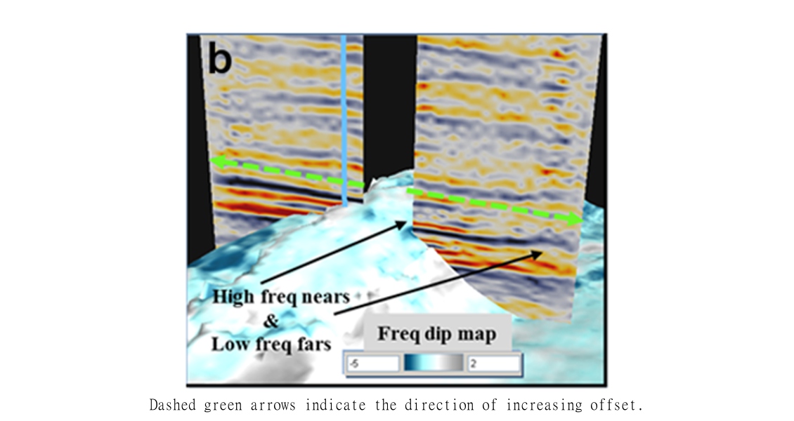
Figure 1b. 3D view of the top of a chalk reservoir. Average frequency dip with offset maps can help to highlight zones of significant multiple interference and can explain why some gather events have more time change on the far offsets than others.
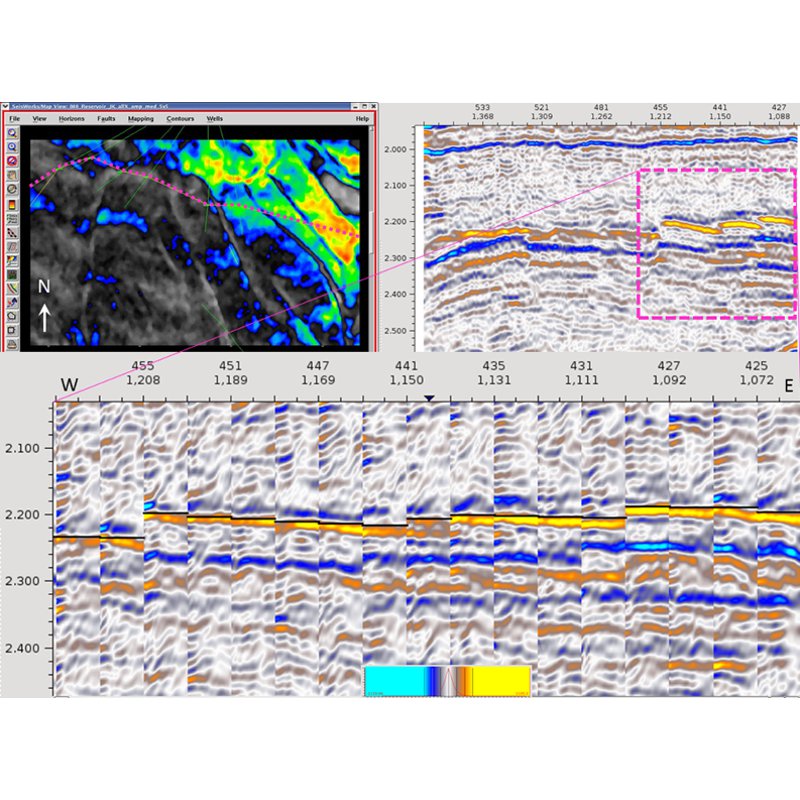 Figure 2. Synchronised map, full stack and gather sections, along the arbitrary line indicated by the pink dotted line. The map shows the RMS amplitude below the black horizon, displayed on top of the gathers. The stack section shows every trace location, the gather section only 1 in 20 of those from the area inside the pink box.Tools that provide real-time interactivity are proving to be key to bridging the stack barrier. Inline, crossline or arbitrary lines displaying both stacked and gather data can now be created by drawing lines on maps that, when dragged from one location to another within a seismic cube, can be used to explore the data volume. Figure 2 is an example of this using Pre-StackPro from Sharp Reflections. All gather traces from this 3D survey are kept in memory by the application allowing interactive pan and zoom, decimation, and even arbitrary line repositioning by the interpreter, giving exceptional access to all the data. These gathers can also be used to restack the stack cross section and even recalculate the RMS amplitude map, on-the-fly, with any change in pre-stack processing parameters. A truly stack <-> pre-stack, linked, sync’d, interpretation environment.
Pre-stack horizons can also be tracked through the volume, often using post-stack horizon times as a guide and gather quality/character attribute maps to focus the cross-section browsing and analysis of the pre-stack data. The time and average frequency dip maps in Figure 1 are examples of these gather character maps being used to understand the geology better and to assess interpretation uncertainty. This is fast becoming a first step ‘health check’ procedure for interpreters preparing to condition their gathers for AVO inversion.
Another way to visualise pre-stack with post-stack data is to turn pre-stack horizons into pseudo post-stack-seismic volumes, with the vertical axis being the gather’s fourth dimension, usually offset or angle, and sample values being amplitude (AVO) , time (TVO) or a time-windowed attribute such as average frequency (FVO). Figure 3, panel a, shows an AVO pseudo post-stack-seismic volume, hung below its guide post-stack-interpreted horizon-time, underneath the original stack section (created using Landmark’s WellSeismicFusion software). The geoscientist can now use the pre-stack data, within their normal post-stack interpretation environment, to challenge and improve ongoing post-stack interpretations, whilst at the same time taking advantage of the fluid and lithology indicators within the data.
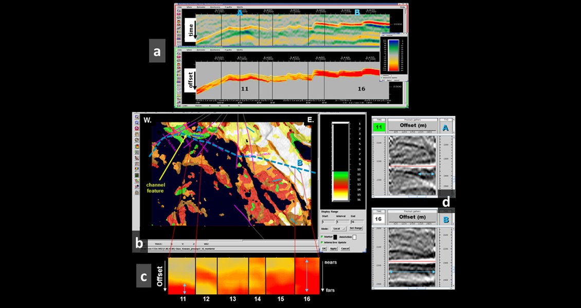
Figure 3. K means, unsupervised classification of an AVO, post-stack volume – into 16 classes. Panel a, shows the arbitrary line from Figure 2 (above) for both the original seismic and the AVO post-stack volume (red is high amplitude). Panel b, is the class map with higher amplitude classes 11 to 16 visible. Panel c, shows the AVO character of traces from those classes, 11 through 16. Panel d shows 2 gathers, A from green class 11 and B from white class 16. See text for a full description.
Figure 4 illustrates the method used. The pre-stack interpretation of the top reservoir (green/blue trough) from the post-stack section [1], seen in the CMP gather [2], is rotated clockwise 90 degrees [3] and written into a new post-stack volume as pseudo seismic traces at the same X,Y location as the original post-stack picks [4] – the vertical axis is now offset instead of time. The top panel shows the ‘AVO’ offset volume from this workflow for comparison with the original seismic data in the bottom panel (blue = highest amplitudes). The interpreter can see immediately how the pre-stack ‘AVO’ changes, on the target horizon, as it moves up the structure from west to east – in the west the ‘AVO’ amplitude has much more of a gradient and a small intercept compared to the east where strong constant amplitudes dominate.
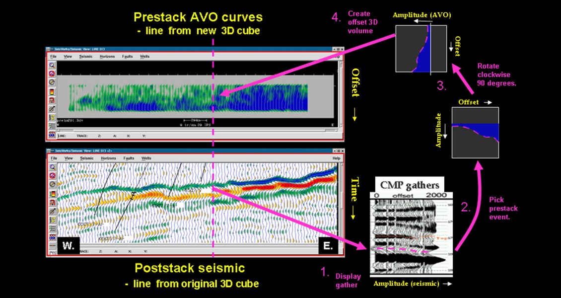
Figure 4. Cartoon showing how a pre-stack horizon can be turned into an amplitude offset (AVO) post-stack volume (where blue is high and grey is low amplitude). See text for a full description.
These pseudo post-stack-seismic volumes can also be mined for interesting character using seismic trace shape classification algorithms, removing any chance of interpreter bias.
Figure 3, panel b, shows a class map from the AVO pseudo post-stack-seismic volume traces, created using the Poststack/PAL application, from Landmark. Looking at the 2 gathers in panel d, and the amplitude around the red line; the gather at location A belongs to the green ‘class 11’ and is interpreted to be part of a channel feature. Class 11 is characterised by a low-intercept and a high-gradient, whereas the gather at location B belongs to the white ‘class 16’, which is characterised by a high-intercept and a low-gradient (panel c). So, we can see that k means, unsupervised classification, combines both intercept and gradient information and, in fact, can find any interesting patterns or anomalies inside AVO/TVO/FVO data, to enhance our understanding of the pre-stack seismic data volume.
Breaking the stack barrier.
By the 1950s scientists and engineers had dispelled the myth of the ‘sound barrier’ and many combat aircraft could routinely break the barrier in level flight. Nowadays, aircraft can transit the barrier without it even being noticeable. In a similar way, the science and the enabling technologies that allow us to breach the stack barrier, to unlock the real value of the data hidden behind the stacks, is available to us now and it is only a matter of time before the commonplace use of gather data becomes ‘unnoticeable’.