As with conventional plays, the economic case for developing and producing an unconventional field is based on how much resource exists, whether it is gas or oil, and how much can be extracted at what cost. The answers for shale plays lie in the volume and maturity of the total organic carbon (TOC) and the ability to create an effective fracture network that will conduct the hydrocarbons to each borehole. This in turn requires an understanding of mineralogy, lithology, relative rock brittleness, natural fracturing and the directionality of in situ rock stresses.
Shale play sweet spots are typically characterised by mid to high kerogen content, lower clay volumes, higher effective porosity, low water saturation, high Young’s Modulus and low Poisson’s Ratio. Using these properties as a guide, reservoir engineers can define a drilling programme that focuses on the best targets in the field and optimises the recovery from each well.
Petrophysical analysis is the starting point, combining laboratory measurements, core data and well logs. Rock physics then establishes the relationship between petrophysical and elastic properties of the formation and enables the creation of synthetics for missing and bad log data. Seismic data analysis moves the analysis beyond well control to the whole field. At the conclusion of the workflow there should be sufficient information about the reservoir character to select optimal drilling locations, as well as orientation and placement
To see the detailed graphics please download our PDF for the print issue available through this link: GEO ExPro Vol. 10 No. 3
Step 1: TOC and Mineralogy
 Poisson’s Ratio computed from P-Impedance and S-Impedance using Jason RockTrace deterministic simultaneous AVO inversion. The plot is overlain with Poisson’s Ratio from logs. The white arrow indicates the reservoir level in the lower Barnett. Low Poisson’s Ratio rocks are more brittle.Determining TOC and mineral composition within the zone of interest is a critical first step in unconventional formation evaluation. The relative quantity and distribution of minerals and TOC are key to understanding the formation, and optimising production from it. For example, certain minerals, such as quartz, are more prone to fracture, while clay tends to fill and close fractures. Large volumes of pyrite can decrease measured resistivity. Kerogen type and maturity determine the oil/gas ratio, and volume establishes whether there is sufficient economic potential to continue the analysis.
The highly laminated nature of most shales presents a challenge for traditional analysis, as they harbour consolidated and compacted parasequences of shallow marine sediment, clay, quartz, feldspar, and heavy minerals. They exhibit ultra-to-low inter-particle permeability, low-to-moderate porosity, and complex pore connectivity.
A stochastic or statistical model is used to estimate relative volume and distribution of TOC and minerals. First, the presence and volume of some constituents are determined directly from core and well log measurements, such as shale volume from gamma ray or natural gamma ray logs and dry clay bulk density from crossplots of porosity and resistivity. These constituents are used as input to the model to estimate relative volume and distribution of TOC and minerals. If mineral composition is well understood, a deterministic approach can be taken instead.
Core data is the optimum control mechanism to validate the model. Passey and Modified Passey methods can be used as a quality control check on TOC volume, and uranium, a strong indicator of TOC, has the same use. The methods work best in shale sections with high clay content and no permeability. If the reservoir is self-sourcing and self-sealing, TOC is directly proportional to the kerogen volume, which can be determined by calibrating log responses to core data for at least one well in the area under study.
Density plays an important role in the analysis, given the disparity between various constituents, with pyrite having high density and a smaller volume and kerogen a larger volume percent than indicated by weight. Core-XRD mineralogy provides bulk-rock mineral weight percent, but excludes porosity and kerogen, whereas volume percent includes all minerals plus kerogen.
After the model is built and validated against well and core data, it can be applied to other wells in the field within the same general lithology. Geoscientists can then compare water saturation, porosity, and mineralogy with confidence.
Step 2: Field Level Lithology
 Map of Interval Velocity Anisotropy from the Fayetteville shale. Colour indicates magnitude of anisotropy; arrow length indicates magnitude of fast velocity. Arrow directions represent azimuths. Initial production from Well Y was three times that from Well X. (Courtesy Southwestern Energy)Once well and core data are interpreted they are combined with seismic data to extend the understanding of rock properties to the space between wells. This allows a better understanding of lithological detail across the field and leads to identification of the most attractive facies.
Shales present several challenges to seismic interpretation. Laminations cause polar anisotropy, distorting seismic data which must be corrected during seismic processing or inversion, and are also below normal seismic resolution, so special averaging must be performed to accurately reflect the composition of the formation. A tie must be interpolated between well and seismic data, such that data at any wellbore can be recreated by the seismic; this well tie is what enables characterisation and modelling of the field away from well control.
Simultaneous AVO inversion produces a deterministic set of rock properties that can be QC’d against core and well log data. The inversion process accounts for AVO anomalies and reduces tuning and interference effects that can be problematic in simple seismic data analysis. Because laminations are below seismic data resolution, Backus averaging is employed to transform them to the seismic scale. Detail is added through a low frequency model generated as part of the inversion workflow.
Geostatistical inversion provides additional layer detail necessary to simulate flow. It simultaneously inverts impedance and lithology, producing more objective and geologically plausible models than other methods. The models have realistic detail, and also include uncertainty estimates. Integrating 3D seismic into geostatistical modelling can be challenging. The physical relationship between petrophysical properties and seismic measurement must be specified directly or by analysing well log data in conjunction with rock
Step 3: Brittleness and Ductility
 PDFs (Probability Density Functions) of predicted volume of quartz vs. predicted brittleness displayed in Jason Facies and Fluids Probabilities™. The five numbered zones each enclose similarly coloured clusters of data points that indicate the different lithotypes.Once TOC, mineralogy and lithology are understood, the formation can be evaluated for relative fracability. Brittleness – the likelihood of fracturing under stress – is key. Ductile shale naturally heals, while brittle silty shale with a quartz fraction is more likely to fracture. Geomechanical properties help determine relative brittleness or ductility, providing valuable input into completion and fracture stimulation design.
A combination of static testing (triaxial compression) and dynamic testing (ultrasonic velocity) establishes a relative brittleness measure. Zones with high Young’s Modulus and low Poisson’s Ratio will be more brittle and have higher reservoir quality (TOC and porosity are both higher).
Calculating Poisson’s Ratio from seismic data is straightforward as it depends strictly on Vp/Vs, obtained from the ratio of P- and S-impedance. Young’s Modulus requires a measure of density, usually unavailable due to the limited range of angles in the seismic data, so it is necessary to evaluate several different potential proxies for density to determine the best one for the particular geology. The starting point, although rarely sufficient, is P-impedance, with other proxies involving a combination of S-impedance, Poisson’s Ratio, and a regression of P-impedance; the method chosen depends on the specific lithology. Core analysis is then used as a real world confirmation at each well location.
Brittleness is a relative not an absolute measure. It is based on a combination of core and sonic data and assumes that fractures open and remain open better in brittle rock. Shale formations are quite distinct from each other and vary in quality internally.
Facies can be identified from deterministic inversions following a Bayesian scheme. The inputs to the process are the inversion outcomes and PDFs (Probability Density Functions) representing the facies to be determined, estimated from log data or analogues. The outputs of the process are probability volumes for each facies and a most-probable facies volume, as shown below.
To see the detailed graphics please download our PDF for the print issue available through this link: GEO ExPro Vol. 10 No. 3
Step 4: Fracture Directionality
 Cross section of the most likely lithology correlated across all of the wells from the Top Barnett to the Top Viola, computed using Jason Facies and Fluids Probabilities. Source: Southwestern EnergyFollowing brittleness analysis, the areas most prone to fracturing should be well understood. The next step is to determine the best well bore direction for optimised conductivity and production.
Productivity is a function of fracture direction, induced fracture extent, network intensity, propensity to sustain fractures, effective conductivity and matrix permeability: all governed by mineralogy and rock stresses, and all evaluated from seismic. Determining these properties improves sweet spot identification, reserve estimation, well placement, completion design, stimulation effectiveness, and production enhancement.
Fractures occur when rock is stressed naturally or with stimulation. Induced fractures run perpendicular to the direction of minimum rock stress, and open fractures created perpendicular to the well bore, typically vertical, provide the best opportunity to drain the area around it. If the formation is incorrectly fracced, the fractures may close, extend into water areas, or ineffectively conduct hydrocarbons.
The three principal components of rock stress allow estimation of how rocks are likely to fracture under stress during fracture stimulation. The vertical stress component is the overburden pressure of the rock on top of the reservoir. Differential horizontal stress components (minimum and maximum) are consequences of tectonics.
The effects of rock stress can be seen on borehole images, with natural fractures quite apparent. Differential effective stress squeezes the borehole causing breakouts in the direction of the minimum stress effect. The structural model from seismic also shows how the rock is stressed, and seismic structural attributes can be used to indicate fractures below accepted seismic resolution. The coherence attribute, used to detect faults or discontinuous features, can pick up swarms of parallel fractures.
Directional stress is determined using azimuthal anisotropy analysis. The distinct layers of organic material in laminated shales exhibit electrical anisotropy – electrical conductivity in one direction different from another. Sand reservoirs have high resistivity (low conductivity) whereas shales have lower resistivity. Anisotropy has a first-order influence on shear and mode-converted PS-waves, which split into fast and slow modes with orthogonal polarisations. Because fractures and faults are mostly in the vertical direction and aligned along the direction of maximum horizontal stress, the result is azimuthal anisotropy (HTI). An azimuthal map can show the direction of the fast component, its magnitude and a measure of the difference between the maximum and minimum velocity, data which helps determine drilling direction, well positioning and hydraulic fracturing strategy.
The differential horizontal stress ratio can be calculated from seismic parameters without any knowledge of the stress state of the reservoir, preferably using wide angle, wide azimuth 3D seismic. Greater differential stress and/or higher fracture density results in greater anisotropy. By mapping the anisotropy at the reservoir level, geoscientists can see the direction, magnitude and difference between the maximum and minimum stress directions. A combination of Young’s Modulus and differential horizontal stress indicates high potential areas for creating fracture networks, optimal drilling locations and best well bore orientation.
Azimuthal anisotropy is typically caused by near-vertical systems of aligned fractures and microcracks, pinpointing higher-potential producing areas. Anisotropic analysis identifies both higher differential stress and natural fracturing, but the difference between them is dependent on the play and cannot be separated mathematically.
Through these analyses, geoscientists can find natural fractures and areas with low anisotropy prone to fracturing. More fracturing may be needed where there are many faults. Effective fracturing determines the production rate and drainage area recovery. Complex fractures appear to be preferable, and drainage is very efficient when a high-relative-conductivity primary fracture is present, rather than a uniform-conductivity network.
Step 5: Planning the Well Trajectory
By this final step in the workflow, there should be sufficient information to determine detailed well placement and fracture stimulation. Planning each well trajectory is an important element of success, given the heterogeneity common in shales.
Target facies, consisting of mid to high kerogen content, low clay and brittle rock, are identified through petrophysical and lithological analyses and refined with brittleness analysis. Because shale is laminated by nature, these targets may vary in height of pay interval and proximity to each other (laterally and/or vertically), requiring adjustments to the well bore trajectory to optimise contact.
Results from rock stress analysis identify the optimal well bore direction for fractures that will remain open and provide effective conductivity to the well bore. Placement of the vertical segment of each well can then be guided by the optimal horizontals in combination with surface considerations.
Each well can be drilled in the optimum stratigraphy throughout its entire length, avoiding water and ductile zones. Known fracture conductivity barriers can be used to separate the well bore from water zones. Stimulation can be managed to limit frac height growth and avoid communications with adjacent water-bearing zones. High clay zones can be mapped so that fracturing is not wasted. Fractures must remain open to be conductive, so proppant may be required to prevent oil and gas from being trapped. To maximise fracture complexity, operators may use closer spacing of perforation clusters with more fracture treatments, small proppants at higher injection rates, closer spacing between laterals, and simultaneously alternate fracture treatments in offsetting wells to focus stimulation energy. Success depends on a strong understanding of the rock properties and rock stresses unique to each field and well.
Specialised Software
Shale plays require special analysis to consistently obtain optimum results from each well. By combining all the well and field data, including cores, well logs and pre-stack 3D seismic data, geoscientists can understand key characteristics that enable them to estimate reserves, place well bores in the most appropriate trajectory and define the overall drilling completion and fracture stimulation programme.
All of this analysis is enhanced and accelerated by specialised reservoir characterisation software for methodical analysis of TOC, minerals, natural fractures, rock stresses, fracture orientation, brittleness and other aspects of the play. Using these tools and methods, geoscientists can make better decisions about where to drill and how to frac, and can better predict economic outcomes.
References
A. Babarsky, D. Gao. “Fracture Detection in Unconventional Gas Plays Using 3D Seismic Data.” SEG 2012.
K.Bandyopadhyay, R. Sain, E. Liu, C. Harris, A. Martinez, M. Payne, and Y. Zhu. “Rock Property Inversion in Organic- Rich Shale: Uncertainties, Ambiguities, and Pitfalls.” SEG 2012 Abstract.
L.K. Britt and J. Schoeffler. “The Geomechanics of a Shale Play: What Makes a Shale Prospective!” SPE Paper 125525, 2009.
M.P. Brown, J.H. Higginbotham, C.M. Macesanu, O.E. Ramirez, and C. Lang. “PSDM for Unconventional Reservoirs? A Niobrara Shale Case Study.” SEG 2012 Abstract.
S. Chopra, R.K. Sharma, J. Keay and K.J. Marfurt. “Shale Gas Reservoir Characterization Workflows.” SEG 2012 Abstract.
C.L. Cipolla. “Modeling Production and Evaluating Fracture Performance in Unconventional Gas Reservoirs.” Journal of Petroleum Technology, September 2009.
D. Denney. “Highlights from Integrating Core Data and Wireline Geochemical Data for Shale-Gas-Reservoir Formation Evaluation and Characterization.” Journal of Petroleum Technology, August 2011.
D. Denney. “Highlights from Whole Core vs. Plugs: Integrating Log and Core Data to Decrease Uncertainty in Petrophysical Interpretation and Oil-In-Place Calculations.” Journal of Petroleum Technology, August 2011.
D. Gray, P. Anderson, J. Logel, F. Delbecq and D. Schmidt. “Estimating In-Situ, Anisotropic, Principle Stresses from 3D Seismic.” EAGE 2010.
M. Haege, S. Maxwell,L. Sonneland, and M. Norton. “Integration of Passive Seismic and 3D Reflection Seismic in an Unconventional Shale Gas Play: Relationship Between Rock Fabric and Seismic Moment of Microseismic Events.” SEG 2012 Abstract.
F. Jenson, H. Rael. “Stochastic Modeling & Petrophysical Analysis of Unconventional Shales: Spraberry-Wolfcamp Example.” 2012.
A. Kalantari-Dahaghi, S.D. Mohaghegh. “Top-Down Intelligent Reservoir Modeling of New Albany Shale.” SEP 125859. Society of Petroleum Engineers, 2009.
R. Kennedy. “Shale Gas Challenges/Technologies Over the Asset Lifecycle.” US-China Oil and Gas Forum Presentation. September 2010.
R. Lewis, D. Ingraham, M. Pearcy, J. Williamson, W. Sawyer, and J. Frantz. “New Evaluation Techniques for Gas Shale Reservoirs.” Reservoir Symposium, 2004.
Q.R. Passey, K.M. Bohacs, W.L. Esch, R. Klimentidis, and S. Sinha. “From Oil-Prone Source Rock to Gas-Producing Shale Reservoir—Geologic and Petrophysical Characterization of Unconventional Shale-Gas Reservoirs.” SPE 131350. Society of Petroleum Engineers, 2010.
D. Themig. “New Technologies Enhance Efficiency of Horizontal, Multistage Fracturing.” Journal of Petroleum Technology, April 2011.
A.N. Tutuncu. “Incorporating Stress Anisotropy in Determining Time-Dependent Rock Properties During Production Optimization and Environmental Monitoring in Shale Reservoirs.” SEG 2012 Abstract.
I. Tsvankin, J. Gaiser, V. Grechka, M. van der Baan, and L. Thomsen. “Seismic Anisotropy in Exploration and Reservoir Characterization: An Overview.” Geophysics, Vol 75, No 5, September-October 2010.
R. Varga, R. Lotti, A. Pachos, T. Holden, I. Marini, E. Spadaford, and J. Pendrel. “Seismic Inversion in the Barnett Shale Successfully Pinpoints Sweet Spots to Optimize Well- bore Placement and Reduce Drilling Risks.” SEG 2012.
P. F. Worthington. “The Petrophysics of Problematic eservoirs.” Journal of Petroleum Technology, December 2011, p. 88-96.