Geomicrobial Exploration
Microbial magic: how medical DNA fingerprinting can de-risk hydrocarbon exploration and production.
Geomicrobial exploration is a novel technique within geochemical exploration. It uses the same base principle of detecting a signal at the surface resulting from vertically moving micro-seepage originating from a subsurface hydrocarbon accumulation. The technology to measure this signal is built on innovations developed over the last decade: firstly, automated DNA fingerprinting and secondly, machine learning algorithms that benefit from the exponential growth of computing power. With these machine learning algorithms, it is possible to unravel tiny differences within terabytes of sequence/microbial abundance data for samples taken above potential hydrocarbon accumulations. This makes it possible to de-risk exploration considerably and lays the foundation for a reliable, non-intrusive, and sustainable technology. The methodology is a cross-innovation from an application in medical sciences where the DNA fingerprint of a cheek swab is an indicator for the presence of specific cancers.
Innovative Techniques for Detecting Micro-seepage
The causal relationship between anomalies and DNA fingerprints above oil and gas fields is micro-seepage. It consists of small (colloidal size) gas bubbles that move upwards solely due to buoyancy with a speed that is > 100m/year at micro-scale. The bubbles are generated in the transition zone of gas to water, when the buoyancy pressure exerted by the gas is greater than the capillary forces in the water, allowing the gas to migrate into the water. Due to the density and viscosity differences, viscous intrusion of petroleum gas into water will appear. As the hydrostatic pressure is very high, the tips of the intruding gas ‘fingers’ will snap-off and form bubbles. Since the drag force that opposes the upward movement of the bubbles is proportional to the radius of the bubbles, while the buoyancy force depends on the cubic radius, colloidal-size bubbles are created. These can come together later to form clusters. This process takes place at the reservoir/seal interface, and in the upper part of a productive shale (Figure 1).
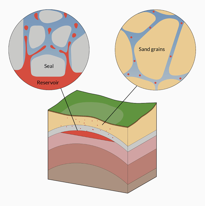
Figure 1: The origin of micro-seepage is the displacement of water with colloids of gas in the lower part of the seal.
Once the bubbles are formed, they move upwards to the surface due to buoyancy (the pressure exerted by the water molecules on a bubble force it upwards). Because this process takes place from nano- to micro-scale, the micro-seepage is negligible in volume compared to ‘normal’ migration of hydrocarbons according to pressure differences and geology (‘Darcy flow’ or secondary migration).
Because of the small volume, micro-seepage is difficult to measure. However, the slight increase in hydrocarbon concentration will influence the ecology of a tiny fraction of the bacteria that live in the subsurface. Some of these metabolise the gas as a carbon source for their growth (e.g., methanotrophs/methanophiles), while others find the new environment detrimental to their growth (methanophobes or methanotoxic). The DNA fingerprinting methodology uses the 16S rRNA gene as a unique genetic indicator for a specific bacterial species. A schematic representation of the steps for DNA fingerprinting is shown in Figure 2. The most difficult and determining step for the quality is the extraction of DNA from the soil. Our methods for this have been optimised during the processing of nearly 10,000 samples that are currently available in our database.
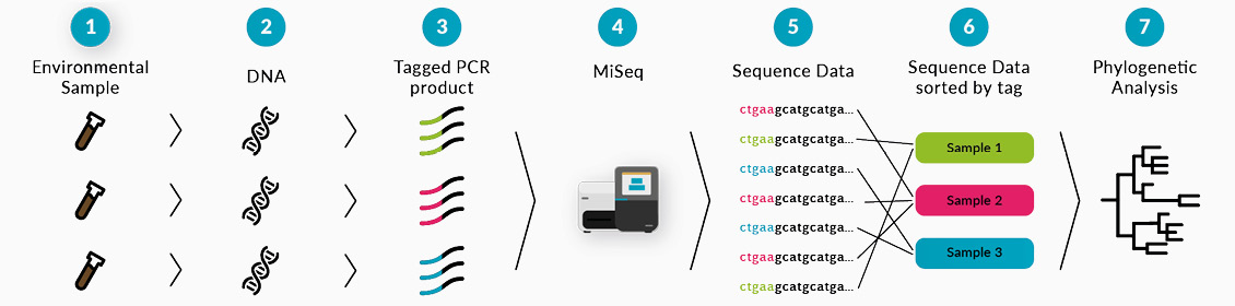
Figure 2: Schematic steps in microbial fingerprinting: identification of which microbes are present in the soil samples and their abundance.
The second innovation used is machine learning to find the ~100 microbial species that indicate oil and gas presence out of the millions of species present in the DNA fingerprint of the soil sample. The power of machine learning lies in the possibility to effectively check all possible combinations to pinpoint the required 100 species (by a ‘deep learning neural network’) and in maximising and extensively testing the predictive capability of candidate models. Training and calibration are followed by validation, which is checking that the predictive accuracy on reserved data samples is correct, as shown in Figure 3. Only when the prediction accuracy is acceptable is the model used to predict new/blind samples, otherwise the predictive capability of the model is improved first.

Figure 3: Extensive testing of predictive capabilities with machine learning.
In the Field, an American Case Study
In recent years, several successful proof-of-concept projects have been carried out which have been published in articles and at conferences and exhibitions. One of these projects was an extensive proof-of-concept pilot carried out in the Bakken and Eagle Ford Shale Formations in the United States. To obtain an accurate prediction of the customer-supplied blinded samples, we used the following workflow (Figure 4), also described in more detail by Te Stroet et al. (2017). Firstly, soil sampling was conducted 1 ft below the surface (half a teaspoon). Next, DNA analysis was undertaken resulting in DNA fingerprints of the microbial ecosystem of each sample. Then modelling and validating of the microbes that determine the hydrocarbon presence was undertaken and finally, mapping and predicting the prospectivity of new samples.
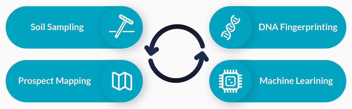
Figure 4: The workflow used to obtain an accurate prediction of samples which were either blinded by a customer beforehand, or when the subsurface potential charge is unknown.
The goal of this project was to investigate whether the technique can distinguish between high and low producers in the Bakken (North Dakota) and Eagle Ford Shale Formations (Texas). In order to do this, 540 samples (Figure 5) were taken above selected high and low-producing wells, subdivided into three different sets: high and low-producing wells in the Bakken oil shale, high and low-producing oil wells of the Eagle Ford, and high and low gas producers of the Eagle Ford. To obtain valid predictions, 200 samples (70 from the Bakken, 30 from the Eagle Ford oil window and 100 from the Eagle Ford gas window) were blinded by the customer after sampling. From 340 non-blinded samples the abundances of all microbes present per sample were analysed using machine learning. The algorithms look for differences above known highly productive wells and wells with known low productivity and then uses these to train a predictive model.
This was done by three modelling loops: 1) an inner loop of non-blinded samples used to correlate DNA fingerprints with known well productivity, also known as the training set; 2) an iterative second loop of non-blinded samples not used for training that are predicted and cross-validated with known well productivity, referred to as the validation set; 3) an outer loop which predicts the productivity of the blinded samples by using the parameters of the second loop. To preserve data integrity, the client applied a randomisation mask to the blinded samples and evaluated the delivered prediction results by removing the randomisation mask. The resulting model achieved an accurate prediction of well productivity of 85% on the blinded samples.
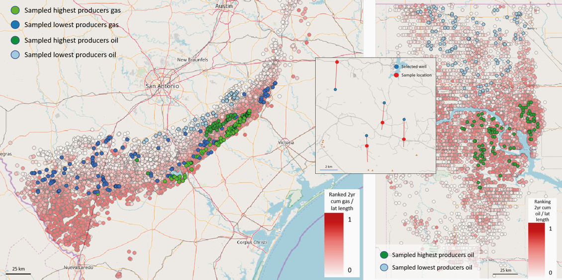
Figure 5: Sample locations of the Eagle Ford Shale (left) and the Bakken Shale (right). Red/white dots show all drilled wells per play, blue/green dots are sampled wells. Inset shows how samples are taken at publicly accessible locations (roads in dark grey) above the well lateral (red lines).
Following this it was necessary to evaluate whether a model trained in one location could be used to predict a different location. To test this ‘exportability’, we used the combined data from the Bakken and Eagle Ford Formations to predict the productivity of one of the other study areas, the Vaca Muerta Basin in Argentina. The result was that the USA dataset (540 samples) predicted the Argentina blinded samples with an accuracy of 83%, despite the study areas being several thousand kilometres apart and in different climatic zones. This means that the selected bacteria are found in both locations, and analysis of their reaction to the presence or absence of microseepage can achieve consistently good results.
Decrease Environmental Impact, Increase Drilling Success
From this exercise we conclude that the large number of shale wells and the public reporting of production information in the USA, make it very suitable to use DNA fingerprints of shallow soil samples to develop a robust machine learning model which predicts hydrocarbon production with an accuracy of around 85%. The potential for application of a trained machine learning model on geographically distant areas is demonstrated. Whilst having local samples and productivity data increases the accuracy of study results, the USA data-trained model provided predictive accuracies above the success threshold when considering Argentina samples. This indicates that in addition to providing a development criterion complementary to other available techniques for existing fields, new fields in non-contiguous areas can also use this innovative and non-intrusive approach for prospect evaluation, de-risking, and initial well selection prior to production data being available. In currently ongoing offshore work, quite different bacterial ecosystems have been found to be present, compared to onshore, and the next phase is to diligently develop and build a corresponding sample database to support further efforts in this area.
References
- Abrams, M.A. (2020) Microseepage vs. Macroseepage: Defining Seepage Type and Migration Mechanisms for Differing Levels of Seepage and Surface Expressions, Search and Discovery, 42542.
- Davis, J.B., (1956) Microbial decomposition of hydrocarbons. Industrial and Engineering Chemistry, vol. 48, no. 9, pp.1444–1448.
- England, W.A. et. al., (1987) The movement and entrapment of petroleum fluids in the subsurface, Journal of the Geological Society, London, Vol. 144, 1987, pp.327–347.
- Klusman, R. W. (1993) Soil gas and related methods for natural resource exploration, New York, John Wiley, 483 p.
- Klusman, R.W., M.A. Saeed (1996) Comparison of Light Hydrocarbon Microseepage Mechanisms. Hydrocarbon migration and its near-surface expression, eds. D. Schumacher and M.A. Abrams, AAPG Memoir 66, pp.157–168.
- Laubmeyer, G. (1933) A new geophysical prospecting method, especially for deposits of hydrocarbons. Petroleum London, vol. 29, 14.
- Price, L.C. (1985) A Critical Overview of and Proposed Working Model for Hydrocarbon Microseepage Report.
- Schumacher, D. (1996) Hydrocarbon-induced alteration of soils and sediments. Hydrocarbon migration and its near-surface expression: AAPG Memoir 66, eds. D. Schumacher, M.A. Abrams, pp.71–89.
- te Stroet et. al. (2017) Predicting Sweet Spots in Shale Plays by DNA Fingerprinting and Machine Learning. URTeC, nr. 2671117.
- Todesco, S. A. (1999) Anomaly shifts indicate rapid surface seep rates. Tulsa, Okla. Vol. 97.1999, 13 pp.68–71.