Recent Advances in Climate Change Research: Part VII – Arrhenius’ Greenhouse Rule for Carbon Dioxide
Here, we investigate the relationship between radiative forcing (heat warming) of carbon dioxide and its concentration in the atmosphere to better understand climate feedback and sensitivity.
In Part II of this series (Recent Advances in Climate Change Research: Part II – Arrhenius and Blackbody Radiation) we referred to Arrhenius’ relationship between radiative forcing (heat warming) of CO2 and its concentration in the atmosphere, and glibly informed you that the effect is logarithmic. However, there is no simple proof as to why this is the case. In this article we investigate this, as it sheds light on understanding climate feedback and sensitivity. We go on to show how the surface temperature changes with variation in CO2 concentration. Our simplifications should only be regarded as the first steps toward getting a feeling of the greenhouse effect.
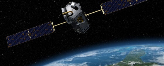
In 2014, NASA launched the satellite OCO-2 (Orbiting Carbon Observatory-2) to monitor CO2 in the Earth’s atmosphere. Source: NASA/John Howard/JPL.
Radiative Forcing
Radiative forcing since 1750. Source: IPCC Working Group 1.
The greenhouse effect is caused by the absorption of longwave, infrared radiation from the Earth by greenhouse gases in the atmosphere. Changes in the concentration of these gases lead to a change in the radiative energy absorbed, and thus a change in the temperature of the atmosphere, leading to a change in its radiation back to Earth. The difference in radiation received by the Earth between two defined conditions is called radiative forcing (Myhre et al., 2013). There are two common examples given in the literature. The first is the forcing believed to be caused by an increase in atmospheric CO2 concentration since pre-industrial times. The second one, obtained from computer climate models, is the forcing produced as a result of doubling the concentration of atmospheric CO2. The forcing can be converted to a mean global surface temperature change by multiplying it by a climate sensitivity parameter which varies between the different models. Radiative forcing is considered a direct measure of the amount by which the Earth’s energy budget is out of balance.
On Arrhenius’ Greenhouse Rule for CO2
The history of CO2 and climate usually starts with Arrhenius’ 1896 paper arguing that increased levels of CO2 could raise global temperatures. Other scientists rejected this assertion, based on their belief that CO2 did not absorb any radiation wavelength that was not also absorbed by water vapor: the atmospheric CO2 level is so small compared to the level of water vapor that its effect would be insignificant. Therefore, for nearly 50 years the scientific consensus stated that CO2 could not affect Earth’s temperature.
However, Arrhenius believed that atmospheric CO2 (and other gases) had an effect on surface temperatures; and he formulated a greenhouse rule for CO2 by stating: “If the quantity of carbonic acid increased in geometric progression, the augmentation of the temperature will increase nearly in arithmetic progression.” The augmentation of the temperature is the change in the rate of heating Earth’s surface (i.e., radiative forcing).
The Keeling Curve is a graph of the changes in atmospheric CO2 concentrations since 1958 taken at the Mauna Loa Observatory, 3,300m above ground level in Hawaii, by the Scripps Institution of Oceanography. The measurements show a steady rise from about 316 ppm in 1959 to 414 ppm in March 2020. The annual fluctuation in CO2 is caused by seasonal variations in CO2 uptake by land plants. Since CO2 is a greenhouse gas, the curve has been interpreted by many climate scientists as a warning signal for global warming. The effect of the outbreak of the coronavirus pandemic declared by the World Health Organization (WHO) on 11 March 2020 is expected to show up in this curve after some time.
To interpret Arrhenius’ statement, we need to recall some basic math. Progressions (also called sequences and series) are numbers arranged such that they form a predictable order; i.e. that given some numbers, we can find the next numbers in the series. A sequence of numbers is an arithmetic progression if the difference between any two consecutive terms is always the same. When the initial term of an arithmetic progression is a1 and the common difference of successive members is d, then the n’th term of the sequence is given by an = a1 + (n−1)d. A sequence of numbers is called a geometric progression if the ratio of any two consecutive terms is always the same. The general form of a geometric sequence is a, ar, ar2, ar3, … where r is the common ratio, and a is a constant. What is of interest to us now is that geometric sequences show exponential growth (or decay), as opposed to the linear growth (or decline) of an arithmetic progression.
Now, according to Arrhenius’ calculations, when CO2 increases in geometric progression – say, from 1 to 2 to 22 = 4 to 23 = 8 … i.e. has exponential growth – the radiative forcing increases (nearly) in arithmetic progression – i.e. shows linear growth. Since logarithmic and exponential functions are inverse functions, equation (1) below suggests itself. In particular, when C/C0 = (1,2,4,8…) then ΔF = (0,1,2,3,…)αln(2).
In Table VII of his paper (see Part II), Arrhenius lists calculations of variation of radiative forcing caused by a given variation of CO2. At latitude 0, CO2 ratios of 1, 1.5, 2.0, 2.5, 3.0 yield temperature increases of 0, 3.1, 4.9, 6.3, 7.2, respectively. We can easily check the validity of Arrhenius’ observation by calculating the constant α for each of his calculations, which we find to be in the range 6.6–7.7 and thus in agreement with the quote we have taken from Arrhenius’ paper. The relationship between concentration and radiative forcing is nearly logarithmic.
Why Logarithmic?
Logarithmic equations for calculating the radiative forcing of CO2 are common. The functional form:
ΔF = α ln(C/C0) [W/m2] (1)
was published by Wigley (1987) using the model of Kiehl and Dickinson (1987). Here, C is the CO2 concentration and C0 is the reference concentration at the beginning of the period being studied. The form in equation (1) was used by IPCC 1990 with coefficient α derived from Hansen et al. (1988). The best estimate based on radiative transfer calculations with 3D climatological meteorological input data (Myhre et al., 1998) is α = 5.35. Even though there is no theoretical basis for formula (1), it has been accepted by the scientific community as a reasonable approximation for the range from 275 ppm to 378 ppm of CO2, the levels from the beginning of the Industrial Revolution to 2005. The logarithmic relationship implies that radiative forcing will rise by roughly the same amount for each doubling of CO2 concentration. Thus, increased concentrations have a progressively smaller warming effect.
Let’s calculate the radiative forcing from the beginning of the Industrial Revolution, C0 = 275 ppm, to October 2019 when C = 408.55 ppm. Equation (1) gives the warming effect ΔF = 2.06 W/m2. That may not sound like much until you multiply by Earth’s total area, which gives a total warming effect of about 1,050 TW – more than 58 times the world’s average rate of energy consumption, which is currently about 18 TW.
The logarithmic dependency is intriguing. Clues of its usefulness are given also in textbooks, usually pointing to the spectroscopic features of the absorption lines. The interested reader may consult Goody and Yung (1989) or Pierrehumbert (2010). More recently, Huang and Shahabadi (2014) have proposed a simpler argument for why we would expect logarithmic dependence for monochromatic radiance, i.e. at a single wavelength.
Do Goats Combat Climate Change?
U make me goat crazy. Source: Alexas_Fotos/Pixabay
All animals emit methane, which can be converted into CO2 equivalents; goats in Norway emit approximately 24 kilotons per year. Since the goat and sheep population is decreasing, the area of cultivated land is also decreasing, to be replaced by bushes and trees. This causes a reduction of approximately 6% in the albedo effect (the difference between cultivated agriculture landscape and the same landscape covered by bushes and trees). So, there are obviously two counteracting effects: the decrease in global temperature caused by increased albedo if, say, five goats keep 1,000m2 clean, compared to the increase in temperature caused by the emissions from the same goats. For simplicity we assume that the goats are only fed by the grass and vegetation they eat. We use the equations derived in this article to obtain a ballpark estimate and compare the two effects. The change in temperature due to change in albedo is ΔTalbedo = TΔα/(4(1 – α)). The change in albedo for the 1,000m2 has to be scaled by the earth’s surface. In addition, we have to correct for the fact that approximately 70% of the incoming solar radiation is reflected by clouds and does not hit the earth’s surface. Then Δα = 0.06 · (1 – 0.7) · 1,000/(5.1 · 1014) = 3.53 · 10-14, leading to a temperature change of ΔTalbedo = 3.65 · 10-12K which of course would have a negligible effect on climate. The five goats emit approximately 1.86 tons of CO2 per year; this represents 1.86/(35 · 109) = 5.31 · 10-11 of the total global yearly emissions. The yearly increase in atmospheric CO2 is (see the Keeling curve) approximately 1.82 ppm/year. From equation (6) we find that the change in temperature is ΔTco2 = 3.71 · 10-13K. We observe that the albedo effect is approximately ten times the CO2 emissions from the five goats. It is of course a very simplified example, where several of the numbers used are not perfect, but we can actually state: goats do combat climate change.
Temperature Increase
A figure in Part VI (Recent Advances in Climate Change Research: Part VI – More on the Simple Greenhouse Model) depicts radiative equilibrium for the Earth system with a single-layered atmosphere. At the surface the downward radiation flux emitted by the atmosphere is F = (β/2) σT4, where we have substituted the atmospheric temperature with the surface temperature according to equation (2) in Part VI. Increasing, say, CO2 concentration by a given amount corresponds to an increase Δβ of the absorption efficiency. The radiative forcing is the radiative response to the forcing agent, taking place quickly without change in temperature; then the energy imbalance imposed on the climate system is:
ΔF = ΔβσT4(β)/2 (2)
Now, since more energy is radiating down on Earth than is radiating back out to space, the planet gets upset; its response is to heat up. Eventually, after decades, a new equilibrium state is reached where the surface temperature has increased by ΔT. Equation (1) in Part VI defines the new temperature as T(β + Δβ). For a sufficiently small perturbation, a Taylor series expansion of T(β + Δβ) yields:
By use of equations (1, Part VI) and (2) above we can eliminate Δβ in equation (3) and obtain the linear relation:
ΔT = λΔF (4)
where λ is the climate sensitivity factor:
λ = T(β)/(S(1 – a)) (5)
We proceed with a cavalier disregard for the observed limitations of the one-layer educational atmospheric model and insert Arrhenius’ rule (1) into equation (4), thereby suggesting that:
ΔT = γ ln(C/C0) [K] ; γ = λα (6)
The Earth is generally regarded as having warmed about 1°C since the beginning of the Industrial Revolution, around 1750, when the global average amount of CO2 was 275 ppm. We can use that temperature T = 15°C (288.15K) as a baseline for estimating the effect of CO2 doubling.
First, calculate from equation (5) the climate sensitivity factor λ = 0.302 km2 W-1. Secondly, calculate γ = λα = 1.61 and insert into equation (6) to find the temperature increase ΔT = 1.61 ln(2) K = 1.12°K. Thus, the simple greenhouse model predicts a global warming of around 1.12°C for a doubling of CO2. This value is too low compared to more advanced models, which allow for positive feedback, notably from the increased water vapor due to increased temperature. A simple remedy for including this feedback process is to posit an additional increase of Δβ to approximate the effect of the increase in water vapor that would be associated with an increase in temperature.
Allowing Δβ to double, the model then predicts ΔT ≈ 2.24°C for a doubling of CO2, roughly consistent with the IPCC understanding that climate sensitivity is somewhere between 1.5–4.5°C of warming for a doubling of pre-industrial CO2 levels.
We await the IPCC’s new assessment of global warming, due in 2021. New computer models predict a warming surge, where equilibrium sensitivity looks to be 5°C. However, in assessing how fast climate may change, the next IPCC report is expected to look to other evidence as well, in particular how ancient climates and observations of recent climate change constrain sensitivity.
Further Reading in the ‘Recent Advances in Climate Change Research’ Series
Recent Advances in Climate Change Research: Part I – Blackbody Radiation and Milankovic Cycles
Martin Landrø and Lasse Amundsen, NTNU / Bivrost Geo
Geoscience will probably play an important role in mitigating carbon dioxide emissions. In part one of this series, we discuss some history and physics behind the topic of climate change including the concepts behind blackbody radiation and Millankovic Cycles.
This article appeared in Vol. 16, No. 2 – 2019
Recent Advances in Climate Change Research: Part II – Arrhenius and Blackbody Radiation
Martin Landrø and Lasse Amundsen, NTNU / Bivrost Geo
In Part II we look at Arrhenius’ seminal 1896 paper and see how it relates to blackbody radiation and absorption of infrared radiation by the atmosphere, taking a closer look at his model of the greenhouse effect.
This article appeared in Vol. 16, No. 3 – 2019
Recent Advances in Climate Change Research: Part III – A Simple Greenhouse Model
Martin Landrø and Lasse Amundsen, NTNU/Bivrost Geo
What would the temperature of Earth be without the atmosphere? By using simple physical models for solar irradiation and the Stefan-Boltzmans law for blackbody radiation, we can estimate average temperatures with and without atmosphere.
This article appeared in Vol. 16, No. 4 – 2019
Recent Advances in Climate Change Research: Part IV – Challenges and Practical Issues of Carbon Capture & Storage
Martin Landrø, Lasse Amundsen and Philip Ringrose
The basic idea behind CCS (Carbon Capture and Storage) is simple, but what are the main challenges and practical issues preventing a more global adoption of this method?
This article appeared in Vol. 16, No. 5 – 2019
Recent Advances in Climate Change Research: Part V – Underground Storage of Carbon Dioxide
Eva K. Halland, Norwegian Petroleum Directorate. Series Editors: Martin Landrø and Lasse Amundsen, NTU/Bivrost Geo
By building on knowledge from the petroleum industry and experience of over 23 years of storing CO₂ in deep geological formations, we can make a new value chain and a business model for carbon capture and storage (CCS) in the North Sea Basin.
This article appeared in Vol. 16, No. 6 – 2019
Recent Advances in Climate Change Research: Part VI – More on the Simple Greenhouse Model
Lasse Amundsen and Martin Landrø, NTNU/Bivrost Geo
We continue the discussion of the simple greenhouse model introduced in Part III.
This article appeared in Vol. 17, No. 1 – 2020