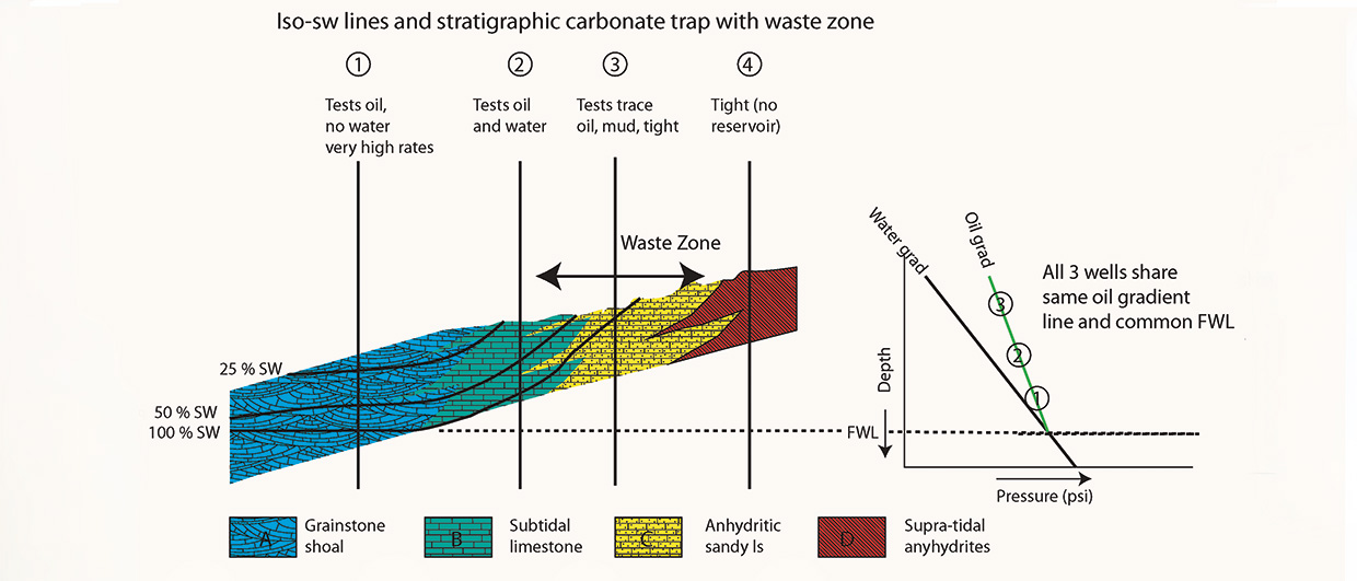
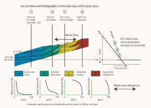
Water saturation (Sw) variation in a stratigraphic trap where test results can be misinterpreted and a commercial field missed. Source: From Dolson (2016) and Coalson et al. (1994).
Hunting for NULFs
Is using well data to hunt for those NULFs (Nasty, Ugly Little Facts!) that lead to breakthroughs in exploration thinking becoming a lost art?
Thomas Huxley (1825-1895), in an 1870 address to the British Association, famously said, “The great tragedy of science is the slaying of a beautiful hypothesis by an ugly fact.” One of the key roles of a geologist is to sort through well and rock information, and to test old-ideas with new-data or to find new-ways to think about old-data.
But are we losing the ability to teach the next generation of geoscientists how to use existing data to get new ideas? Are we allowing 3D computer or seismic images to trump hard work analyzing well data? Understanding how to interpret oil and gas shows in the context of migration and entrapment using well data is hard work. Well reports have to be read, logs and log analysis investigated, and mud logs, head space gas readings, biostratigraphical and petrography analysis must all be integrated to be fully understood. None of this is glamorous work, but it has to be done.
Understanding shows
Consider this case: Company A had a multi-disciplinary team screening its acreage to decide what to retain. A block acquired in a company merger has a dry hole on it. Seismic shows the dry hole is a small 4-way closure. Maturation maps show it is over 50 km away from mature source rock. Concluding that no oil had migrated into this area, and with no other visible structural traps, the acreage was dropped. Company B was thrilled, because the ‘dry hole’ actually had 3.5m of pay on logs in a porous Jurassic sandstone. They recognized a seismically defined up-dip stratigraphic trap – and subsequently drilled the 1.4 Bbo-in-place Buzzard Field discovery (Carstens, 2005; Dolson, 2016; Ray et al., 2010). The more careful analysis of the ‘dry well’ invalidated the pessimistic migration model and also de-risked reservoir issues.
Sound unusual? It isn’t. A major complaint I hear from all oil companies is that far too many young geoscientists are drawn immediately to 3D seismic or computer simulations without a firm understanding of how to use well and geochemical data to test models.
Two of the ground-breaking papers on understanding oil and gas shows were those of Schowalter (1979) and Schowalter and Hess (1982). Few younger geoscientists are even aware of these papers or understand how to distinguish a show along a migration pathway from live oil within an accumulation, or how to use water saturation (Sw) to determine position in a trap. Vavra et al. (1992) and Hartmann and Beaumont (1999) are two additional papers that should be required reading for any geoscientist looking to understand how to interpret test data and shows in the context of capillarity and position in a column.
Consider Figure 1 (below), a carbonate shoreline trap with degrading reservoir quality due to pore throat reduction up-dip into waste zones. How to interpret the test results depends not just on the sequence in which the wells are drilled, but the ability to integrate the petrophysical data. If well 3 is drilled first, it may be declared a dry hole with high Sw that looks wet in porous but low permeability rock. Drill well 1 first, and optimism abounds, but results in disappointment on the up-dip offset. Well 2 is more problematic. The key to recognizing a potentially large field here is the pressure and rock data, which shows the different facies as part of the same column. The fact that oil is actually recovered in wells 2 and 3 shows a trap with a column. If knowledge exists of the pore-throat sizes or capillarity, an astute geoscientist might be able to quantify the elevation above the free water level and speculate on where better facies might exist that would produce water-free oil, potentially even down-dip of wells 2 and 3.
Key skills
Learning to understand test and show data to seek out those elusive ‘NULFs’ requires re-thinking porosity and permeability in a way that quantifies pore throat distribution. In Figure 1, the porosities may be similar in wells 1-3, but with radically different pore throat sizes and saturations at any point in the trap. Pittman (1992) and Winland (1972) determined a way to calculate pore throat sizes statistically using readily available permeability and porosity data. Once pore throat sizes are estimated, and with reasonable assumptions of interfacial tension, wettability and subsurface water/hydrocarbon densities, pseudo-capillary pressure curves can be made to estimate saturation-height functions. An example of this is shown for the Pennsylvanian carbonates in Colorado’s Four Corners area in Dolson (2016). In addition, rocks with similar pore size distributions will have similar flow units. Understanding the geometry of these flow units and their saturation variations at any given point in a column is critical to understanding development scenarios (Ebanks et al., 1992; Gunter et al., 1997).
Without these skills as part of their fundamental ‘tool kit’, young geoscientists are doomed to miss a lot of plays, inappropriately plug a lot of wells and leave oil behind pipe for others to find. Worse, they confuse oil or gas-water contacts with free water levels, not understanding that micro-porous rocks may have 100% Sw well above spill point of the trap.
Understanding pressures is another key skill. Integration of pressure data is critical to understanding connectivity and position in a trap. Figure 2 illustrates seal recognition from pressure data and how to use the slopes of the curves to calculate fluid density. However, in the absence of other data the pattern shown in the image could also be interpreted as the result of hydrodynamic flow.
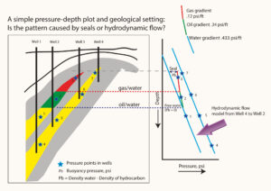
In 37 years of consulting, I have seldom seen geoscientists make potentiometric surface maps to quantify the impact of hydrodynamic flow in tilting oil and gas contacts, despite the landmark work of Hubbert (1953), Dahlberg (1982, 1995) and England (1994). Many geoscientists do not recognize the presence of tilted oil and gas columns caused by an upward flow of expelled waters from over-pressured areas towards the basin flanks. Numerous recent examples of tilted contacts in deep basin settings show the potential to underestimate trap size due to tilting (Ferrero et al., 2012; Muggeridge and Mahmode, 2012; O’Connor and Swarbrick, 2008; Riley, 2009; Robertson et al., 2013).
FIS and migration modeling
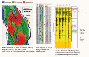
Many advances have been made in capturing new information in old wells, particularly Fluid Inclusion Stratigraphy (FIS) (Dolson, 2016 and Hall, 2008). Mud log, mud gas and cuttings data provide the first step in detecting hydrocarbons but in some cases shows are suppressed and hydrocarbons missed. Fluid inclusion data often picks up subtle shows, or key information like temperature of emplacement of fluids, API gravity, salinities, proximity to pays, migration pathways, seals and even biomarkers useful for source to oil correlation.
The example shown in Figure 3 is from a well where there were no mud log or sample shows. FIS data, however, showed abundant migration and evidence for micro-seepage at the surface. These data provide new insight plays and prospects.
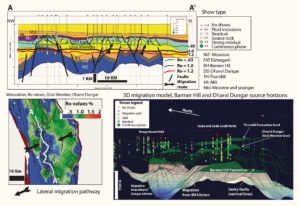
Modern petroleum systems software performs very powerful 4D and 3D migration and maturation modeling – but how rigorously are the models tested against well data? Calibration is essential, and requires carefully analyzing and capturing well information in ways that can be displayed in the models, as in Figure 4. Proper shows analysis is a time-consuming but critical role for a geologist.
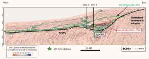
Another useful technique is to quickly and qualitatively convert seismic depth images into reservoir-seal pairs (in meters of seal capacity) based on amplitude variations.(www.zetaware.com). Figure 5 models migration off the west coast of Africa. While only a crude representation of the real subsurface data, these solutions give a good feel for how migration might work, and can be developed quickly.
While much more sophisticated models can be run using more quantitative rock property modeling, pressures, hydro-dynamics, and other data, they are time-consuming and expensive to build, particularly if in a 3D seismic volume. Worse, all models involve multiple assumptions on fluid phase, seal capacity, fault leakage, pressures, etc., adding complexity to the model but not necessarily insight. A good discussion of the main benefits and pitfalls to petroleum systems migration modeling is that of He (2016).
The young geologist skill set
Just some of the skill sets needed for young geoscientists are summarized here:
- Understand the rocks: go look at cores and cuttings.
- Think of rocks in terms of pore throats, capillarity, Sw and position in a trap.
- Understand pitfalls in log analysis or formation damage due to unusual minerals and/or shaliness.
- Build and refine oil and gas show databases that can be mapped and visualized quantitatively.
-
Post-appraise key dry holes carefully, looking for anomalous shows.
-
Simulate migration scenarios, first conceptually, and then with appropriate software.
-
Build appropriate seal and pressure maps and integrate them into migration models.
-
Supplement mud log shows with FIS, thin sections or classic fluid inclusion studies to help ground-truth migration and entrapment.
-
Systematically use geochemical analysis of source rocks and reservoired hydrocarbons to try to understand migration pathways and source to oil correlations.
About the Author
John Dolson holds a B.A. in Natural Sciences from Colorado College and an MSc. in Earth Science from Colorado State University.
John has over 37 years of experience in oil and gas exploration both domestically and internationally, with Amoco, BP, his own company (DSP Geosciences and Associates, LLC) and as a Senior Geological Advisor to Delonex Energy.
As well as his commercial ventures, John is passionate about education and is currently an Adjunct Professor at the University of Miami, teaching petroleum geology.
A past Vice-President of AAPG, John remains active in many geoscience societies.
Image caption: John Dolson.
Acknowledgement:
Cairn India Pty and Ion Geophysical have been particularly helpful for permissions to use some key figures. The author is also indebted to Zhiyong He and Jeff Corrigan for review of this manuscript and many productive discussions over the years regarding calibration and construction of petroleum migration models.
References
Carstens, H., 2005, Buzzard- a discovery based on sound geological thinking: GEO ExPro, p. 34-38.
Coalson, E. B., S. M. Goolsby, and M. H. Franklin, 1994, Subtle seals and fluid-flow barriers in carbonate rocks, in J. C. Dolson, M. L. Hendricks, and W. A. Wescott, eds., Unconformity Related Hydrocarbons in Sedimentary Sequences, v. 1: Denver, Colorado, Rocky Mountain Association of Geologists, p. 45-59.
Dahlberg, E. C., 1982, Applied Hydrodynamics in Petroleum Exploration: New York, New York, Springer Verlag, 161 p.
Dahlberg, E. C., 1995, Applied Hydrodynamics in Petroleum Exploration, 2nd Edition: New York, New York, Springer Verlag, 295 p.
Dolson, J., 2016, Understanding Oil and Gas Shows and Seals in the Search for Hydrocarbons: Switzerland, Springer International Publishing Switzerland, 486 p.
Ebanks, J., N. H. Scheihing, and C. D. Atkinson, 1992, Flow units for reservoir characterization, in D. Morton-Thompson, and A. M. Woods, eds., Development Geology Reference Manual: AAPG Methods in Exploration Series 10: Tulsa, Oklahoma, American Association of Petroleum Geologists, p. 282-285.
England, W. A., 1994, Secondary migration and accumulation of hydrocarbons, in L. B. Magoon, and W. G. Dow, eds., The Petroleum System – from source to trap: Tulsa, Oklahoma, The American Association of Petroleum Geologists, p. 211-217.
Ferrero, M. B., S. Price, and J. Hognestad, 2012, Predicting water in the crest of a giant gas field: Ormen Lange hydrodynamic aquifer model: Society of Petroleum Engineers, v. SPE 153507, p. 1-13.
Gunter, G. W., J. M. Finneran, D. J. Hartmann, and J. D. Miller, 1997, Early determination of reservoir flow units using an integrated petrophysical method: Society of Petroleum Engineers, v. SPE 38679, p. 1-8.
Hall, D., 2008, Fluid Inclusions in Petroleum Systems, in D. Hall, ed.: AAPG Getting Started Series No. 15, American Association of Petroleum Geologists.
Hartmann, D. J., and E. A. Beaumont, 1999, Predicting reservoir system quality and performance, in E. A. Beaumont, and N. H. Foster, eds., Exploring for Oil and Gas Traps: Treatise of Petroleum Geology, Handbook of Petroleum Geology, v. 1: Tulsa, Oklahoma, American Association of Petroleum Geologists, p. 9.3-9.154.
Hawkins, J. M., D. L. Luffel, and T. G. Harris, 1993, Capillary pressure model predicts distance to gas/water, oil/water contact: Oil and Gas Journal, p. 39-43.
He, Z., 2016, All models are wrong, some are useful-Best practices in petroleum system analyis, in Z. He, ed., PSA webinar 3: Important factors in charge risking, https://www.youtube.com/watch?v=GWMcLMlTiD8.
He, Z., and T. Berkman, 1999, Interactive charge modeling of the Qatar Arch petroleum systems, AAPG Hedberg Conference on multi-dimensional basin modeling, Colorado Springs, Colorado, American Association of Petroleum Geologists.
Hubbert, M. K., 1953, Entrapment of petroleum under hydrodynamic conditions: American Association of Petroleum Geologists Bulletin, v. 37, p. 1954-2026.
Muggeridge, A., and H. Mahmode, 2012, Hydrodynamic acquifer or reservoir compartmentalization?: American Association of Petroleum Geologists Bulletin, v. 96, p. 315-336.
Naidu, B. S., S. D. Burley, J. Dolson, P. Farrimond, V. R. Sunder, V. Kothari, and P. Mohapatra, in press, Hydrocarbon generation and migration modelling in the Barmer Basin of western Rajasthan, India: lessons for exploration in rift basins with late stage inversion, uplift and tilting, Petroleum System Case Studies, v. Memoir 112: Tulsa, Oklahoma, American Association of Petroleum Geologists.
O’Connor, S. A., and R. E. Swarbrick, 2008, Pressusre regression, fluid drainage and hydrodynamically controlled fluid contact in the North Sea, Lower Cretaceous, Britannia Sandstone Formation: Petroleum Geoscience, v. 14, p. 115-126.
Pittman, E., 1992, Relationship of porosity and permeability to various parameters derived from mercury injection-capillary pressure curves for sandstone: American Association of Petroleum Geologists Bulletin, v. 76, p. 191-198.
Ray, F. M., S. J. Pinnock, H. Katamish, and J. B. Turnbull, 2010, The Buzzard Field: anatomy of the reservoir from appraisal to production: Petroleum Geology conference series 2010, p. 369-386.
Riley, G., 2009, Supergiant fields in an overpressured lacustrine petroleum system: the South Caspian Basin, AAPG 2009 Distinguished Lecture Series, Tulsa, Oklahoma, American Association of Petroleum Geologists, p. 32.
Robertson, J., N. R. Goulty, and R. E. Swarbrick, 2013, Overpressure distributions in Palaeogene reservoirs of the UK Central North Sea and implications for lateral and vertical fluid flow: Petroleum Geoscience, v. 19, p. 223-236.
Schowalter, T. T., 1979, Mechanics of secondary hydrocarbon migration and entrapment: American Association of Petroleum Geologists Bulletin, v. 63, p. 723-760.
Schowalter, T. T., and P. D. Hess, 1982, Interpretation of subsurface hydrocarbon shows: American Association of Petroleum Geologists Bulletin, v. 66, p. 1302-1327.
Vavra, C. L., J. G. Kaldi, and R. M. Sneider, 1992, Geological applications of capillary pressure: a review: American Association of Petroleum Geologists Bulletin, v. 76, p. 840-850.
Winland, H. D., 1972 Oil accumulation in response to pore size changes, Wyburn Field, Saskatchewan, Amoco Production Company report F72-G-25 (unpublished), Tulsa, Oklahoma, p. 20