Gravity for Hydrocarbon Exploration
Can an unexplored sedimentary basin be unravelled by gravity? How can gravity in cross-disciplinary workflows estimate the base of salt domes and gas saturation in shallow sedimentary traps ? Read on!
Gravity. It’s not just a good idea. It’s the Law. Gerry Mooney (1977)
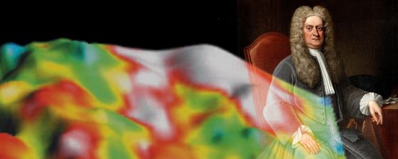
 Portrait of Sir Isaac Newton, c. 1715–1720Thanks to Newton’s Law of universal gravitation, you are safely standing on earth and not flying off into space. The gravitational attraction between two masses increases as their mass expands and decreases as the distance between them grows. For you, this means that you are one mass and mother Earth is another mass – luckily a big one, which attracts you.
From the geological viewpoint, all subsurface rocks are part of the earth’s mass. They cause an attraction on a test-mass, spring-mounted in a gravimeter, the instrument that measures gravity. Just the size of a car battery, it can be located on seismic vessels, aeroplanes or simply on the ground. Tiny deviations from the average gravity force caused by density variations in subsurface rocks are called gravity anomalies. The density of a rock relates to its mineral composition and pore space: sediments, for example, possess low densities, increasing with compaction towards crystalline rocks like granites. Higher on the density scale are mafic rocks like gabbros and basalts; and densest of all are ultramafic mantle rocks.
 Figure 1: Gravity modelling in practice: The hand-hold pointer is at the boundary between top basement and sediments; move it upwards through positions 1 to 3 and the calculated gravity anomaly is changed. The aim is a match with the observed gravity.Gravity anomalies are a composite expression of all the subsurface densities and as such contain a clue to the subsurface geology. The task of an interpreter is to find a reasonable density distribution that matches the gravity anomalies and other geological data. This procedure, known as gravity modelling, can be done simply along a profile or in a more advanced fashion on gridded or triangulated surfaces or even using voxels. Once a basic subsurface geometry has been established and density ranges for the expected rocks are set, the fun begins: grab a body or a point in the model, move it with your cursor, see the immediate change in the gravity in your program and play this game towards a model that matches the gravity (Figure 1).
Alternatively, you can let an inversion algorithm do the work, by telling the program which points it is allowed to move, or which density it can change, and it will find the solution with the best gravity match. This leads to a familiar concern regarding the inherent ambiguity in gravity interpretation, since both unrealistic and reasonable models can generate exactly the same gravity anomaly. The most important strategy to tame the ‘beast’ of ambiguity is to utilise constraints, such as the geometry of layers interpreted from seismic, densities from geological databases, or geological models or analogues. Gravity will always provide a solution space, hopefully narrow enough to provide the missing piece of the puzzle. It can be used to supplement seismic data and geological models with unknown quantities or to create an initial coarse structural model of an unexplored basin.
Let’s look at three important tasks where gravity can make an impact in hydrocarbon exploration.
Basin Structure in Early Exploration
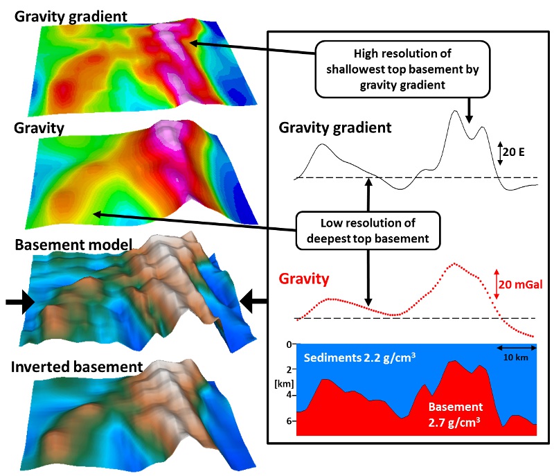 Figure 2: Synthetic model of a highly faulted basement in 3D and on a profile (location shown by large black arrows), with calculated gravity (Gz) and vertical gradient (Gzz). Inverted top basement obtained from inversion of calculated gravity Gz (Parker inversion; GEOSOFT Oasis Montaj).Early basin exploration suffers from a lack of geological information due to scarce seismic coverage. Gravity interpretation can address open questions of basin geometry, sedimentary thickness and direction of structural trends, as illustrated in the synthetic model in Figure 2, consisting of crystalline basement and sediments, where the clue is the contrasting density.
Gravity anomalies and vertical gradients have been computed, the latter representing a highpass filtered gravity version, which enhances details of the shallow structure better than the gravity anomaly itself. The top basement is heavily faulted at all depths and its appearance on the gravity data illustrates the decaying resolution capability with increasing depths: all peaks forming the shallowest part of the basement high are clearly visible on the gravity gradient, which as such provides an excellent tool for top basement mapping. However, fault blocks in the deeper part of the basin (left section of the profile) are smeared together. The same loss of detail occurs when inverting the calculated gravity for top basement, solely based on the pre-defined density contrast between sediments and basement. Nevertheless, the gravity data give a clear idea of the shallowest and deepest parts of the basin as well as the main structural trends, which are related to those of the overlying sedimentary strata. This is useful for 2D seismic survey planning, both ensuring a suitable angle of the lines to the structures and focusing on the most interesting parts of a basin.
The level of detail unravelled depends on the quality of the gravity data, as noise causes artificial anomalies to merge with real ones. For offshore areas, gravity data from satellite altimetry covering the entire world is freely available, or in enhanced quality from contractors. Onshore, the options are airborne or ground gravity data.
In well explored areas, better gravity data should be available, as shown in Figure 3 from the Gjesvær Low in the south-western Barents Sea. The almost triangular depression was identified as a prolongation of the salt-bearing Nordkapp Basin by gravity and only later confirmed by seismic.
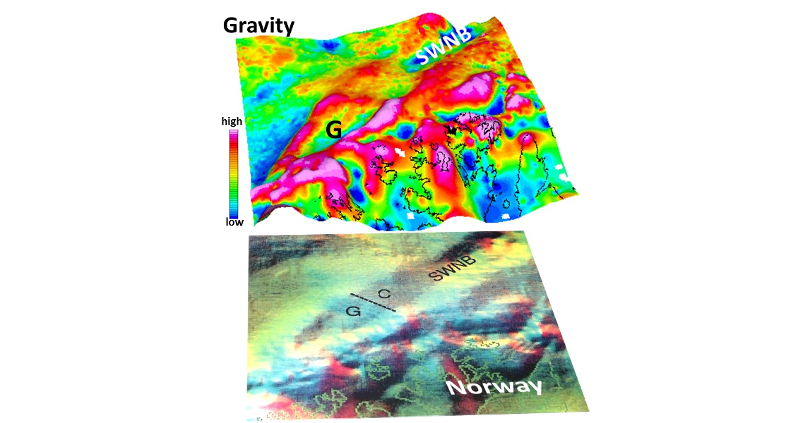
Figure 3: What was hard to see in 1994 is clearly identified on a modern composite data representation, when the small sedimentary basin Gjesvær Low (G) was found to be a continuation of the Nordkapp Basin (SWNB), south-western Barents Sea. Gravity anomalies from a 20-year-old survey are compared to recent results: (upper) modern data (Olesen et al.) in 3D shows vertical gravity gradient draped over the gravity anomalies (GEOSOFT Oasis Montaj); (lower) original display (modified from Johansen et al., 1994.
Modelling of Complex Salt Structures
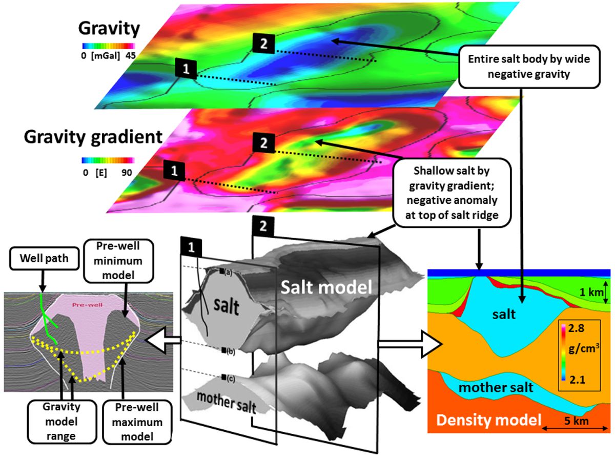 Figure 4: Salt model derived by integrated seismic and gravity interpretation (modified from Stadtler et al., 2014 and Hokstad et al., 2011).The development of a realistic model for some salt diapirs can be a hard nut to crack for seismic imaging, but gravity data can help to define the edge and base of the salt. Figure 4 gives an example from the ‘Uranus’ salt dome in the Norwegian Nordkapp Basin, which was interpreted by combined seismic and gravity gradiometry.
The seismic profile illustrates the lack of reflectors at the base of the salt and presents minimum and maximum salt extension models from the pre-well interpretation. Well data proved the minimum model wrong and, after the acquisition of new gravity and gravity gradiometry data, the density model was developed using sedimentary boundaries and top salt from seismic interpretation and densities from wells.
Salt forms a negative density contrast against surrounding rocks, thus generating a negative gravity anomaly. The vertical gravity gradient, Gzz, senses the shallowest part of the salt, as can be seen by the way the salt ridge lines up with the lowest values of Gzz (dark green and blue). The gravity Gz is wider and smoother as it is also sensitive to the deeper parts of the salt body. This difference in sensitivity is used to address different depth regions during the inversion of Gz and Gzz in order to yield thickness estimates of cap rock, depth to base salt and thickness of mother salt. Modifications in density and salt thickness were used to span the solution space for the base salt, as shown on the seismic profile.
Imaging salt on seismic can benefit from gravity in different phases. Survey planning makes use of early gravity models for optimal orientation and the subsequent seismic processing for quality control of seismic velocities. The velocities can be converted to a density model, which should result in matching gravity anomalies. Finally, seismic interpretation can be improved in an interactive loop with gravity modelling and inversion, as shown in Figure 4.
Shallow Lithology and Gas Mapping
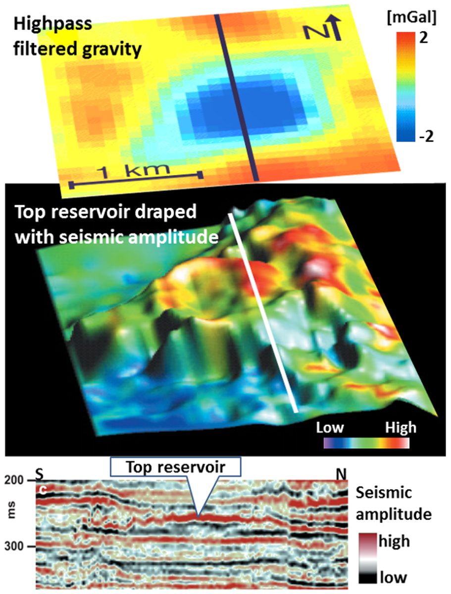 Figure 5: Negative gravity anomaly (blue) indicating a density deficit at a shallow seismic closure, possibly caused by shallow gas (modified after Bauer and Fichler, 2002).It is well known that reservoir monitoring can estimate alterations in gas saturation through density changes observed on repeat gravity surveys. The same effect can be used in exploration to estimate gas saturation in shallow targets, combining the interpretation of 3D seismic and high resolution gravity data.
On Figure 5 a distinct gravity low is seen at the same location as a small seismic closure topped by a seismic bright spot. A detailed density model was constructed from interpreted seismic surfaces and densities from wells, leaving the density of the reservoir as unknown. Gravity modelling was then used to estimate the density within the closure, resulting in values that could indicate either gas-filled sand or a lithology change. When the gas saturation changes, there will be a corresponding linear change in density, which can be combined with seismic to lead to a more precise prediction of gas saturation. This handy connection can only be applied to shallow targets as the resolution of gravity anomalies decays with depth. Furthermore, high quality gravity or gravity gradiometry data are a pre-requisite for such applications.
After this excursion into the world of gravity, hopefully you will feel tempted to include these data in some of your workflows. A final important argument for gravity data is its low cost. Satellite altimetry and country-scale data are often free of charge, and even high resolution gravity data cost only a minor percentage of a seismic budget. Wisely used, serious savings may be achieved with regard to optimally placed seismic surveys in early exploration, and, where applicable, a better constrained seismic interpretation.