Supercomputers for Beginners – Part III. GPU-Accelerated Computing
Many TOP500 supercomputers today use both CPUs and GPUs to give the best of both worlds: GPU processing to perform mathematically intensive computations on very large data sets, and CPUs to run the operating system and perform traditional serial tasks. CPU-GPU collaboration is necessary to achieve high-performance computing.
I changed my password everywhere to ‘incorrect’. That way when I forget it, it always reminds me, ‘Your password is incorrect.’ Anonymous
To greatly simplify, a computer consists of a central processing unit (CPU) attached to memory. The CPU executes instructions read from this memory. One category of instructions loads values from memory into registers and stores values from registers to memory. The other category of instructions operates on values stored in registers – adding, subtracting, multiplying or dividing the values in two registers, performing operations like ‘or’, ‘and’, or performing other mathematical operations (square root, sin, cos, tan, etc).
Until 12 to 15 years ago, CPUs improved in speed mainly by increasing the frequency of their clocks, from MHz speeds to 1 GHz and on to 3–4 GHz. At this point speed stopped advancing, since if the frequency gets too high, the chip can actually melt from the excessive power/heat, unless cooled down. To improve speed, CPU manufacturers added more CPU cores onto the same CPU chip. Each core could work on different tasks so that the user experiences a faster computer. This is where parallel computing first entered the compute scene in a big way. But the CPUs again hit a physical barrier since the size of the chip grew with the number of cores, and the power and heat started to rise again.
For geophysicists and other scientists running big simulations, CPUs were no longer fast enough to get the computing work done. The answer to the challenge was to put GPUs (graphics processing units) on the video card as a companion to the CPU in computational tasks.
GPU developments were primarily driven by the demand for more awesome video games. In order to support the need of physical simulations, GPUs have now advanced significantly enough to do mathematical computations. They can crunch more numbers per minute than CPUs as they have thousands of cores for number calculations. GPUs in addition use less energy per computation than CPUs. Every computer, smartphone and tablet has GPUs in it.
GPU-Accelerated Computing
GPU-accelerated computing is the use of a GPU together with a CPU to accelerate applications, offering increased performance by offloading compute-intensive portions of the application to the GPU, while the remainder of the code still runs on the CPU. From the perspective of the user, the application simply runs significantly faster.
CPU-GPU collaboration is necessary to achieve high-performance computing. Known as heterogeneous computing (HC), which intelligently combines the best features of both CPU and GPU to achieve high computational gains, it aims to match the requirements of each application to the strengths of CPU/GPU architectures and also achieve load-balancing by avoiding idle time for both the processing units. Novel optimisation techniques are required to fully realise the potential of HC and to move towards the goals of exascale performance.
A simple way to understand the difference between a CPU and GPU is to compare how they process tasks. A CPU consists of a few cores optimised for sequential serial processing, while a GPU has a massively parallel architecture consisting of thousands of smaller, more efficient cores designed for handling multiple tasks simultaneously.
Solving a computational problem on a GPU is in principle similar to solving a problem using many CPUs. The task at hand must be split into small tasks where each task is performed by a single GPU core. Communication between the GPU cores is handled by internal registers and memory on the GPU chip. Instead of programming using message passing, special programming languages like CUDA or OpenCL provide mechanisms for data exchange between the host CPU and synchronising the GPU cores.
A modern supercomputer system may then in practice consist of a large number of nodes, each holding between 2 and 32 conventional CPUs as well as 1–4 GPUs. There will usually also be a high-speed network and a system for data storage. The software for this system can be written using a combination of conventional programming languages, like C or C++, combined with a message passing system for parallelisation of the CPUs and in addition CUDA or OpenCL for the GPUs. All of these components must be tuned and optimised for best possible performance of the total system.
The fastest GPU-enabled supercomputer on the TOP500 list, where it is number two, is the Titan Supercomputer at Oak Ridge National Lab (see Supercomputers for Beginners – Part II). Fitted with 299,088 CPU cores and 18,688 Nvidia 2880-core Tesla K20 GPU accelerators, it achieved 17.59 PFlop/s on the Linpack benchmark. Titan is the first major supercomputing system to utilise a hybrid architecture. The second fastest, Piz Daint, number seven on the list, is installed at the Swiss National Supercomputing Centre (CSCS) in Lugano, Switzerland.
Seismic Imaging: RTM
Reverse time migration (RTM) is an industry standard algorithm used to generate accurate images of the subsurface in complex geology. Although RTM has been in use since the 1990s, its applications have steadily widened with increased access to computational power. Because of RTM’s computational intensity, each important step in its development was linked to a significant increase in computational power. Examples include moving from 2D to 3D RTM, from acoustic isotropic to acoustic anisotropic, and from low to higher resolution. In the future, we expect to see quantification of uncertainty in combination with RTM imaging.
Over the last few years, we have seen a shift towards the use of GPUs in seismic data processing and imaging – in particular, RTM. The bulk of the computational cost stems from simulating the propagation of waves inside the earth. The simulation process involves solving differential equations that describe the wave propagation under a set of initial, final and boundary conditions and a velocity model of the subsurface.
In RTM, two wavefields, one from the seismic source and one from the receiver array, are simulated in 3D in the computer. By using a finite-difference approximation of the wave equation, the source wavefield is modelled forward in time whereas the wavefield measured at the receivers is modelled backwards in time. The image is calculated by summing the time correlation of these two wavefields. The wave equation currently used is acoustic with some kind of anisotropy thrown into the model. The space-derivatives of the wave equation can be calculated in the space-domain by using various difference approximations, or more accurately, in the wavenumber domain using so-called pseudo-spectral methods. The space-domain method currently dominates due to the high cost of the wavenumber domain method, which requires 3D Fourier Transforms. However, efforts are being made to develop and implement faster wavenumber domain approaches to RTM. RTM is applied to every shot in a seismic survey. Much effort is paid to keeping data movement to a minimum or to localise it as best as possible – whether it is I/O or message passing.
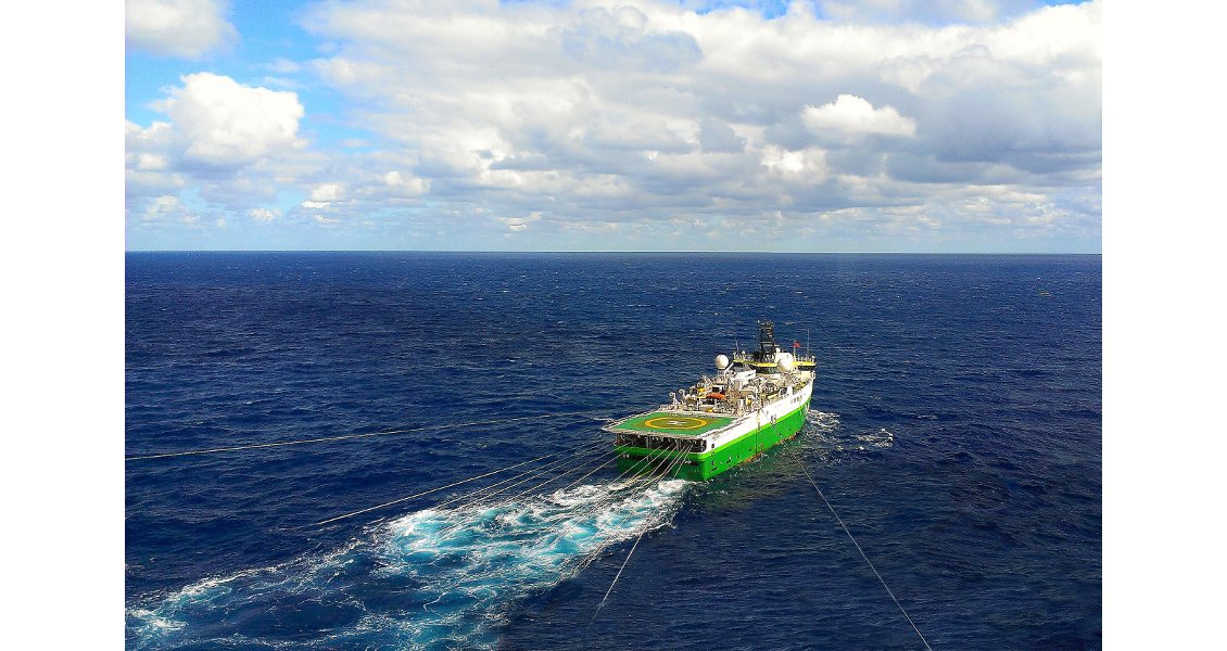
The amount of data collected by seismic vessels continually increases – all needing processing by supercomputers. (Source: Polarcus)
Increasing Volumes of Data
Two trends will affect how RTM is applied in the future: firstly an increase in algorithmic complexity, and secondly an increase in the volume of acquired seismic data to be imaged.
Elastic migration, based on the elastic, anisotropic wave equation, with attenuation, provides a more accurate physics model and ultimately will lead to more accurate subsurface images. However, this would dramatically increase the cost of an already expensive computation. The RTM solution then will require larger grids, and will increase both data parallelism and FLOP requirements. More advanced forms of anisotropy will increase the model space, and lower the operations per memory read. Further, to handle attenuation will require additional memory. The immediate consequence of elastic migration is that the compute power required for such algorithms increases, irrespective of the data size.
Until 2015, the trend in seismic data acquisition was to collect more and more data using larger vessels with more streamers, with the objective of further improving imaging and inversion. In particular, the number of sources and receivers in seismic surveying seems to have increased approximately by a factor of 10 every 10 years. Although oil prices took a nose dive from the second half of 2014, leading to difficult market conditions for the international seismic acquisition business, other parts of the seismic market are less affected by the spending downturn, especially data reprocessing and imaging services and specialised technologies (e.g., reservoir monitoring and ocean bottom seismic). Over longer time periods, the trend that we have seen – an increase in the volume of acquired seismic data – is expected to continue. Geophysicists will acquire more and more data – more azimuths, more density, more channels, more frequencies, with longer recording times and at increased resolution – with evergreater efficiency. Our desire to process data at the resolution they are acquired is forcing huge increases in processing, storage and networking requirements.
These trends impact geophysicists. To come up with innovative, useful solutions to the seismic imaging challenge, at one end we need to master wave equations and their numerical solutions, and at the other end to understand heterogeneous computing. As we make imaging more sophisticated we need to make algorithms run even faster. And, as we increase the sophistication of the numerical imaging method, the complexity of the software implementation and optimisation also rapidly increases. These challenges will keep geophysicists, computer architects, programmers and researchers busy for many years to come.