Supercomputers for Beginners – Part II
Energy companies need ever larger computers. This article is the second of three articles giving an introduction to supercomputers . Here, we look at the design of parallel software.
Beta: Software undergoes beta testing shortly before it’s released. Beta is Latin for ‘still doesn’t work’. Unknown
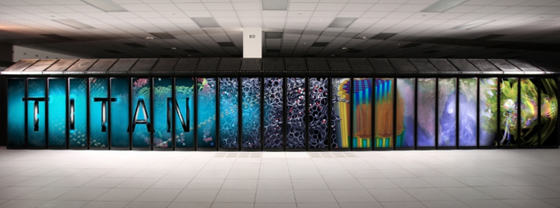 Titan is a supercomputer built by Cray at Oak Ridge National Laboratory. In November 2012, Titan held number one position on the TOP500 list with 18,688 nodes and 552,960 processors. It relies on a combination of GPUs and traditional CPUs to make it today the world’s second most powerful supercomputer, with peak performance of more than 27 petaflops. Titan also has more than 700 terabytes of memory. (Courtesy of Oak Ridge National Laboratory, U.S. Dept. of Energy)Most supercomputers are multiple computers that perform parallel processing, which is well suited for modelling, simulating and understanding many complex, real world phenomena. Historically, parallel computing has been considered ‘the high end of computing’, referring to high capability and high capacity computing, communication and storage resources. It has been used to model difficult problems in many areas of science and engineering. Today, however, a greater driving force in the development of faster computers is provided by commercial applications that require processing of large amounts of data in very advanced ways.
Embarrassingly Parallel Solutions
In parallel computing the problem is divided up among a number of processors. The figure below shows the basic computer layout.
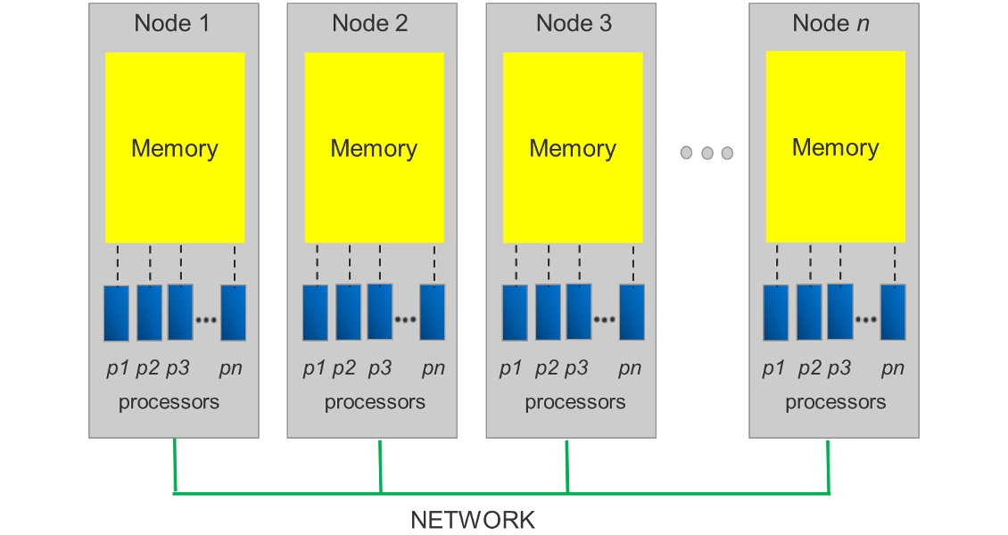
As a rough simplification, the modern supercomputer is divided up into nodes. Each node may have multiple processors which are the hearts of the node. Each processor has access to memory on its node – but does not have access to the memory on the other nodes. Communication of information can occur between processors within or across nodes. Communication across nodes takes place through a high-speed network, but is usually considerably slower than communication within a node. Data storage has to be accessible from all nodes in order to input and output data. In order to benefit from a supercomputer, the programs need to utilise the resources of multiple nodes in parallel. The network connects the nodes to make larger parallel computer clusters.
The art of parallel programming is identifying the part of the problem which can be efficiently parallelised. In many cases this can be straightforward and simple, such as in the processing of seismic data. Seismic data consists of a (large) number of records, and very often a single or a small number of records can be processed independently.
A simplistic example of this kind of processing is the application of various filter operations. The problem is solved by distributing a small number of records to each processor which performs the filtering. This is usually refered to as an embarrassingly parallel solution and, as the name suggests, does not require much sophistication, but a suprisingly large number of problems can be solved by this approach. The gain in computer time needed to solve this kind of problem can be measured by the speedup, which is the ratio of computer time needed to solve the problem using a single processor to the time needed to solve the problem on N processors. For embarrassingly parallel problems the speedup is largely equal to the number of processors used. If each filter operation takes 0.001 second and we want to filter one million records, then a single processor would use 1,000 seconds, while a small supercomputer system with 1,000 processors would need only one second. This way of solving parallel problems is thus highly efficient and simple to implement.
Message Passing Interface
However, in many cases the problem at hand cannot be split into completely independent sub-problems, and some sort of communication must take place between nodes. A common example is a problem where each processor is assigned an independent computation, but where the results from all processors must be combined to form the solution.
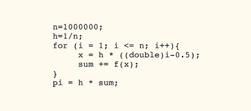 Table 1: An excerpt from a program written in the C language to compute the area under a curve defined by the function f(x)=4/(1+x^2) in the interval [0,1] using the rectangle (midpoint) method; n is the number of rectangles used and h is the width of each rectangle. The third line is the start of a loop doing the area computation and i is a variable looping from 1 and up to n. The expression i++ means that i is incremented by one for each time the loop is executed. The last line computes the final answer, which in this case is the first few digits of the famous number, pi.A simple example of such a problem is the evaluation of an area under a curve. Numerically, this is usually solved by dividing the area up into small rectangles: computing the area for each rectangle and then summing together all individual rectangle areas. Table 1 shows an excerpt from a C program performing this computation on a single processor. Basically the programmer has used a loop to perform the computation of the area of each small rectangle, starting with the first rectangle and sequentially adding together all rectangles to form the total area.
Solving the same problem in a parallel way on a supercomputer with many processors requires some tools not present in conventional programming languages. Although a large number of computer languages have been designed and implemented for this purpose, one of the most popular approaches consists of using a conventional programming language, but extending the language with a small collection of functions capable of sending and synchronising data or messages between processors, a so-called message passing interface or commonly referred to as MPI. It turns out that by using this simple approach a large number of parallel problems can be efficiently programmed.
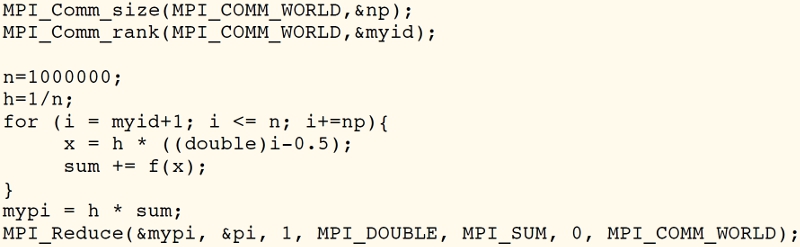 Table 2: The parallel version of the program shown in Table 1. The two first lines are calls to the MPI system returning the number of processors participating (the variable np) and a unique id (the variable myid) for each processor. The variable myid is a number between 0 and the number of processors. The loop in the fifth line is almost the same as for the program in Table 1, but each processor only computes a subset of all rectangles and stores the resulting sum in the variable mypi. The expression i+=np increments the loop variable i by np for each iteration of the loop. The MPI Reduce call in line number 10 adds together all results from each processor and returns this number to processor number 0. In the last three lines, processor number 0 prints the result.The example given in the first table can be parallelised by the computer code shown in Table 2. We see that the addition of only three lines turns the conventional program into an MPI parallel program. At the start of the computation a copy of the program starts execution on each of the processors we have available. The two first lines are calls provided by the MPI system and provide each of the executing programs with information on the total number of processors (the variable np) and a unique number in the range 0 to np identifying each processor.
Let us assume we have a system where np equals 1,000 and that the number of rectangles is equal to one million. The program then works by numbering the rectangles used in the computation from 1 to 1,000,000, and processor number 0 computes the sum of the areas for rectangles number 1, 1001, 2001… and so on up to one million. Processor number 1 does exactly the same, except it computes the sum of the areas for rectangles number 2, 1002, 2002… and so on. When each processor has finished computing their sum, a single MPI Reduce call will combine the sums from each of the 1,000 processors into a final sum. The speedup for this kind of problem is directly proportional to the number of processors used. Running the program in Table 2 using 100 million rectangles on 12 processors gives a speedup of about 11.25, which is roughly what one would expect, allowing some time for overhead. However, if we increase the number of processors to 120 we will only get a speedup of about 40. This seems puzzling until one realises that 120 processors involve 10 different nodes, since the particular machine used for the test runs is equipped with 12 processors per node. The Reduce call then involves communication between 10 nodes. In general, communication between processors on different nodes takes more time than communication between nodes on the same processor.
Balancing Communication
Not all problems can be split up into independent sub-problems. Often large simulation problems involving the solution of differential equations require large amounts of memory to hold intermediate results exceeding the available memory on each node, or the number of numerical operations is so large that the problem has to be split into smaller parts, or domains, in such a way that each processor is able to deal with each of the domains. This is known as domain decomposition. Each of the smaller domains will usually depend on other domains, and an important issue then becomes the interchange of information at the domain boundaries. Each processor, working on a single domain, requires information from other processors.
Hence, some form of communication needs to take place. We have already seen how the MPI system can be used to pass information between processors via the Reduce call shown in the second table. There are in addition a number of calls which can be used to send data from one processor to another. In practice these are relatively easy to use, but the logic and structure of programs rapidly become complicated if the pattern for information exchange is non-trivial. We also learnt that communication between processors on different nodes is expensive in terms of computer time. Hence an important issue is the balance between computing and communication.
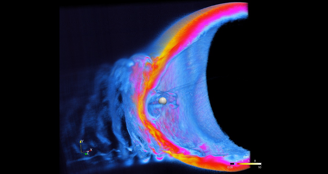
NASA’s supercomputing resources have enabled them to exceed previous state-of-the-art magnetospheric models. The figure shows a snapshot from a 3D simulation of the Earth’s magnetosphere. The plasma density shows formation of helical structures in front of the magnetosphere. The structures lead to turbulence, which in turn amplifies the adverse effects of space weather on Earth and its technological systems. In this project, a typical simulation ran for over 400 hours across more than 4,000 cores on NASA’s Pleiades supercomputer. (Courtesy Homa Karimabadi, University of California, San Diego/ SciberQuest; Burlen Loring, University of California, Berkeley).