Integrating Data Types for Reservoir Characterisation
From microscopic core analysis of the wellbore to seismic data measurements of rock properties between wells, a multidisciplinary team is essential when solving exploration and production problems in complex reservoirs.
Traditionally, oil industry disciplines, namely geology, geophysics, petrophysics, rock physics and engineering, have educated their respective professionals to concentrate on their designated fields and only bring in other disciplines if necessary to achieve a particular result. It is common knowledge in the oil industry that increasingly complex reservoirs require more elaborate solutions in order to effectively and efficiently produce. On the technology side, what this often means is integrating data from different disciplines in order to arrive at a more accurate and meaningful reservoir description.
This article presents an example from Oklahoma in the complex reservoirs of the Mississippi Lime and clearly demonstrates that an integrated team approach to solve exploration and production problems should be adopted as a routine practice. This philosophy is gaining significant traction due to the complexities of unconventional shale plays which defy easy solutions on a regular basis. The industry-wide recognition of this fact is exemplified at the cross-disciplinary URTeC conference, now in its third year and growing fast.
Case Study Data:
Seismic and Logs
The Mississippi Lime is a relatively new tight oil play emerging in north-central Oklahoma and may extend into Kansas. The unit is known to contain abundant natural fractures and be hydrocarbon-charged, therefore the exploration strategy is to find zones with enhanced porosity and natural fractures.
Geomechanical formation properties were calibrated from seismic inversion with vertical and horizontal log suites. (Note that a full petrophysical and rock physics study that included core data was performed and used to calibrate but these topics are beyond the scope of this article.) The vertical logs show that the upper portion of the Mississippi Lime has low Thomsen’s gamma (ratio of vertical to horizontal shear velocity), meaning that it does not contain Vertical Transverse Isotropy (layering) anisotropy, and has a low closure stress gradient, suggesting it is a good candidate for hydraulic fracturing. Along the lateral well, the seismic-derived geomechanical stiffness volume (in this case, Young’s modulus) shows the toe half of the well to be softer, or more ductile, than the heel (lower Young’s modulus values). This is confirmed by the LWD gamma ray log, which shows higher gamma ray readings in the toe half of the well, thus indicating increased shale content. Coincident with this, the Formation Micro-Imager (FMI) fracture log shows the highest natural fracture density in the heel, in the stiffest sediments, with fracture density decreasing toward the toe.
Geomechanical rock properties from seismic inversion (dynamic Young’s modulus) followed by well log-based facies inversion to enhance resolution. Logs are identified on lateral and vertical wells as are tops (on right). For horizontal scale, the lateral is 1,460m long. For vertical scale, the Mississippi Lime (including Kinderhook and Pierson) is about 60m thick. (Source: ION Geophysical)
Microseismic
The microseismic data are in two clusters because there was a 230m stretch in the middle of the lateral that was not completed. However, given this natural division, there still are distinct differences between the toe and the heel clusters. The toe cluster has a larger overall vertical spread with large magnitude events occurring in the upper Mississippi Lime, as well as below the Woodford, and small magnitude events occurring close to the wellbore. The heel cluster is the opposite – it has most of the large magnitude events close to the wellbore with few events outside that zone. We suspect this difference in behaviour is related to the ductility of the sediments in those two areas, but further investigation is needed.
The FMI log shows that the Mississippi Lime, and to a lesser extent the Woodford Shale, is highly fractured, whereas the other surrounding formations are not fractured. These fractures are oriented almost due east (Fast Shear Azimuth) although there is some azimuthal rotation with depth. The Woodford Shale has high TOC (kerogen log) and is the source rock for this hydrocarbon system, including gas shows in the clastic sands of the shallower Pennsylvanian deposits.
Vertical section view through vertical pilot hole and two laterals. The microseismic events are sized by magnitude, show focal planes, and are coloured by Hudson event type (open = purple, close = blue, shear + open = red, shear + close = orange, undefined = green). All events are from the lower of the two laterals. Logs from one vertical well are labelled on the figure. (Source: ION Geophysical)
Anisotropy from Full-Azimuth Seismic
Another element to bring into the Mississippi Lime characterisation is azimuthal velocity anisotropy, as measured from full-azimuth seismic data. Seismic P-wave energy travels faster parallel to fractures and slower when perpendicular to fractures, provided the fractures are not cemented (i.e. open) and especially if they are filled with fluids. Therefore, under these circumstances, azimuthal gathers will show decreased traveltime in the direction of fractures and increased travel-time perpendicular to fractures. The azimuth of fracturing can thereby be determined and the difference between Vfast and Vslow directions (known as PP velocity anisotropy) is proportional to fracture density (and/or fracture openness), as long as the formation lithology and stress conditions do not vary over the measurement area. This anisotropy can be calibrated with fracture logs, thus giving an aerial fracture density map.
The map below shows distinctly different conditions on either side of the major north-east-trending fault to the east of the well pad. To the east of the fault, the anisotropy is higher (3-8%) and a large portion of the azimuths are in an easterly direction (which is the orientation of maximum horizontal stress). There is significant local variation, presumably in response to local fracturing. In addition, the Vfast velocities are lower in magnitude than on the west side of the fault. The situation on the west side of the fault, therefore, seems to indicate that fracture density is low over much of the region except for the area to the south of the southern lateral. This correlates well with data from an FMI log in the lateral wellbore, which shows high fracture density in the heel and low fracture density in the toe.
PP Vfast (base colours) with PP velocity anisotropy vectors overlain for the Woodford. Top colour bar is anisotropy magnitude from 0-8% (for vector colours), lower colour bar is Vfast magnitude from 14,000 ft (4,267m)/sec to 19,500 ft (5,944m)/sec. Wellbores used in the survey are shown in left centre. Note that PP anisotropy is significantly higher on east side of the fault. For scale, the left lateral is 1,460m long. (Source: ION Geophysical)
Assembling the Data
Bringing these concepts together, we assemble a multitude of data types in plan view to see how they fit together and to determine what conclusions can be drawn. The first observation is that the PP and PS anisotropy indicators (which are the base layers) appear to be telling similar stories, and that is that fracturing decreases from south to north along these two laterals. This message is confirmed by the FMI image log on the left lateral. In fact, the FMI can be calibrated to this anisotropy information, giving a rough idea of fracture density away from the wellbores. Associated with this is the LWD gamma ray log in the lateral which, as we have already seen, appears to have responses proportional to rock ductility. Increases in rock ductility are also coincident with decreases in velocity anisotropy and fracturing.
The microseismic data clearly shows the changes in behaviour of the heel and toe groups of events which appear to be related to the amount of seismic-scale faults, with more faults in the heel which is the brittle portion of the well. The heel grouping of microseismic events was clustered at the wellbore level, but in map view these events are shifted to the left, or west, of the wellbore. This grouping is concentrated near several small faults in this area, and also extends towards the area in the leftmost wellbore with the highest fracture density. All of this is consistent with the hypothesis that this portion of the well is more brittle and contains a higher density of fractures and seismicscale faults, which in turn leads to larger magnitude microseismic events.
Conversely, a different situation exists at the toe of these laterals where we have more shale and thus more ductility. This leads to fewer seismicscale faults and fewer fractures. As a consequence, the microseismic data is more scattered with smaller magnitude events in close proximity to the wellbore. Further investigation of the locations of the high magnitude events that appear to be scattered at some distance from the wellbore indicates these events preferentially occur along or in close proximity to seismic-scale faults, many of which are above or below the Mississippi Lime and Woodford Shale units. Thus, hydraulic fracture fluids in this portion of the lateral sought preexisting fractures, reactivating them and creating fluid pathways outside of the reservoir layer, which is something completion engineers attempt to avoid.
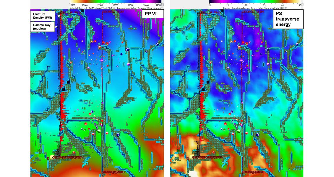
Left basemap shows PP Vfast (brighter colours=slower velocities), right basemap shows PS transverse energy, also referred as C-wave transverse energy (bright colours=large magnitude). Each figure shows two lateral wells; left well shows LWD gamma ray log (dark grey) and FMI fracture density (red); right well shows microseismic events with their associated focal planes, sized by magnitude and coloured by Hudson event type (open=purple, close=blue, shear + open=red, shear + close=orange, undefined=green). Fault traces (in 3D) from seismic fault detection are in green. For scale, the left lateral is 1,460m long. (Source: ION Geophysical)
More Data Integration
Therefore, as a result of this integration of data sets from a variety of sources, we are able to explain the rock and fracture properties of this reservoir. The next step in this workflow is to integrate this information with completions data to explain differences in breakdown pressure, time-transient pressure response (specifically the leak-off component), and instantaneous shut-in pressure (ISIP). Associated with this, an integral part of the evaluation of microseismic responses is time series data for bottomhole pressures, slurry rates, and proppant concentrations for each stage, which enables completion engineers to evaluate the effectiveness of induced fractures. However, each of those topics have complete storylines by themselves and so are beyond the scope of this article.
Nonetheless, this case study clearly illustrates how individual data types typically provide a piece of the reservoir puzzle. However, none by themselves comes remotely close to providing the information needed to make intelligent decisions about where and how to drill and produce a hydrocarbon reservoir. Multidisciplinary integration of all the available data is essential to understand and efficiently exploit the tight, heterogeneous mudstone reservoirs common in today’s unconventional shale plays.