The world’s largest pipe organ was built between May 1929 and December 1932 by the Midmer-Losh Organ Company of Merrick, Long Island, New York. It weighs 150 tons, boasts seven manuals and has 1,439 stop keys, 1,255 speaking stops, 455 ranks, and 33,112 pipes! The most impressive stop on the organ would have to be the 16 ft Ophicleide, which is the world’s loudest stop. This stop has six times the volume of the loudest train whistle. Source: Flickr/Nethercutt.
Broadband seismic technology and beyond, Part I: The drive for better bandwidth and resolution
Once a new technology rolls over you, if you’re not part of the steamroller, you’re part of the road. One such technology is broadband seismic. Want to be part of the steamroller or the road? In a series of articles, we give you an introduction to what broadband seismic has to offer.
Part I: The drive for better bandwidth and resolution
Technology presumes there’s just one right way to do things and there never is. – Robert M. Pirsig (1928–), American writer and philosopher
Most people think of broadband with regard to telecommunications, in which a wide band of frequencies is available to transmit information. This large number of frequencies means that information can be multiplexed and sent on many different frequencies or channels within the band concurrently, allowing more information to be transmitted in a given amount of time (much as more lanes on a highway allow more cars to travel on it at the same time).
In seismic exploration broadband refers to a wider band of frequencies being recorded than in conventional seismic exploration. In the marine case the conventional acquisition system is said to give a useable bandwidth of typically between 8–80 Hz, whereas broadband seismic systems are claimed to give useable frequencies from as low as 2.5 Hz up to 200 Hz or more for shallow targets. On land, marine vibrators today can produce signal frequencies down to 1.5 Hz.
The seismic acquisition system consists of the source system and the receiver system. But in the following discussion we are not going to discuss the technologies behind land or marine acquisition systems; instead, we will give an introduction to resolution and the benefits of hunting in particular for the low frequencies.
In the articles that follow this one, we will present the seismic vendor’s new broadband solutions – a combination of leading equipment, unique acquisition techniques and proprietary data processing technology. With reference to the quote at the start of this article, it is fair to state that there is not one right way to do things. Each of the vendor’s solutions has unique capabilities.
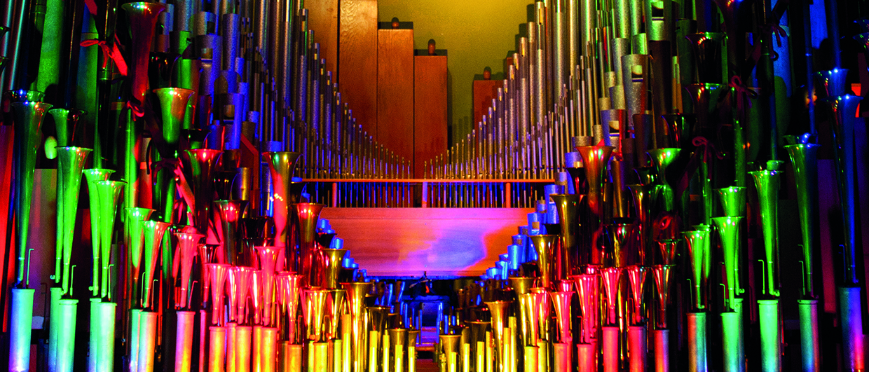
Organ pipes
Did you know that organ pipes have gone through a technology development similar to that for broadband seismic? The frequency f of an organ pipe is f = v/ λ, where v is the speed of sound in air (340 m/s) and λ is the wavelength. Let L be the length of the pipe. The longest possible wavelength equals 2L and 4L for open and closed pipes respectively. The maximum wavelength thus is λ = 4L, and the corresponding minimum frequency equals f=v/4L.
One of the biggest organs in the world is the Boardwalk Hall Auditorium organ in Atlantic City. It is equipped with 33,112 pipes, and the biggest pipe has a length of 64 ft. This is an open pipe so the corresponding lowest frequency is around 8 Hz. A closed pipe of the same length would give a lower frequency of 4 Hz.
But the story does not stop at 4 Hz. The lowest produced note is obtained by combining a stopped 64 ft and stopped 422/3 ft pipe to produce a resultant 256 ft pipe which gives 2 Hz! This is far below the threshold of the human ear, which is approximately 16 Hz. So what is the point in this focus on low frequencies for organ pipes? Can we feel the low frequencies directly on our body, or is it a combination of hearing and body feeling?
Anyhow, there is a strong similarity between the design of big organ pipes and today’s developments in broadband seismic. As geophysicists, we would be thrilled if our marine seismic system produced frequencies truly from 2 Hz and upwards. We would want to activate all the pipes of the organ in Atlantic City, and especially the big pipes! The low frequencies are of particular interest for deep imaging, inversion and high-end interpretation.
Temporal resolution

Improving bandwidth and resolution has been a priority since the early days of the seismic method – to see thinner beds, to image smaller faults, and to detect lateral changes in lithology. Although sometimes used synonymously, the terms bandwidth and resolution actually represent different concepts. Bandwidth describes simply the breadth of frequencies comprising a spectrum. This is often expressed in terms of octaves.
Commonly referred to in music, an octave is the interval between one frequency and another with half or double its frequency. As an example, the frequency range from f1 to f2>f1 represents one octave if f2=2f1. The range from 4 to 8 Hz represents one octave of bandwidth, as do ranges 8–16Hz, and 16–32Hz. Also, the range from f1 to f0 < f1 represents one octave if f0=f1/2.
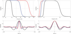
In a classic empirical study, Kallweit and Wood (1982) found a useful relationship between bandwidth and resolution. For a zero-phase wavelet with at least two octaves of bandwidth, they showed that the temporal resolution TR in the noise-free case could be expressed as TR = 1/(1.5 FMAX), where FMAX is the maximum frequency in the wavelet. Other definitions are possible, but for two octaves or more of bandwidth the clue is that one can approximately relate temporal resolution to the highest, and only the highest, frequency of a wavelet. This leads to some very useful and quite accurate predictions. Examples are that wavelet breadth is TB = 1/(0.7 FMAX) and peak-to-trough is TPT = 1/(1.4 FMAX) .
Figure 1 demonstrates the expected improvement in resolution associated with increasing FMAX. We see that when the maximum frequency value is increased while holding the minimum frequency FMIN fixed, sharper temporal wavelets are obtained. Meanwhile, the right side of the figure shows three more temporal wavelets where the FMIN value is changed while holding FMAX fixed. We see that the main lobe shows hardly any change while the side lobes diminish as FMIN is lowered. Thus, filling in the low frequencies gives wavelets with less pronounced side lobe amplitudes. It is attractive because it is smoother, and with less side lobe energy in the wavelet it is unlikely that a small-amplitude event will be lost amid the side lobes from neighbouring, large-amplitude reflections.
Resolution and wavelength
The classic definition of resolution, given by the famous geophysicist Bob Sheriff, is the ability to distinguish two features from one another.
The seismic method is limited in its ability to resolve or separate small features that are very close together in the subsurface. The definition of ‘small’ is governed generally by the seismic wavelength, λ = v/f. Geophysicists can do little about a rock’s velocity, but they can change the wavelength by working hard to change the frequency. Reducing the wavelength by increasing the frequency helps to improve both temporal/vertical and spatial/horizontal resolution. Resolution thus comes in two flavours. The temporal resolution refers to the seismic method’s ability to distinguish two close seismic events corresponding to different depth levels, and the spatial resolution is concerned with the ability to distinguish and recognise two laterally displaced features as two distinct adjacent events.
Figure 2 depicts two similar layers separated by interfaces. The measurable seismic signals that they produce may show as separate, distinguishable signals when they are well separated – a condition we call ‘resolved’. When the interfaces are close together, however, their effects on the seismic signals merge and it is difficult or maybe impossible to tell that two rather than just one interface is present – this condition we call ‘unresolved’. The problem of resolution is to determine how to separate resolved from unresolved domains.
The yardstick for seismic resolution is the dominant wavelength λ. A much used definition of ‘resolvable limit’ is the Rayleigh limit of resolution: the bed thickness must be a quarter of the dominant wavelength. This resolution limit is in agreement with conventional wisdom for seismic data that are recorded in the presence of noise and the consequent broadening of the seismic wavelet during its subsurface journey. The dominant wavelength generally increases with depth because the velocity increases and the higher frequencies are more attenuated than lower frequencies.
The λ/4 limit is by many considered the geophysical principle regarding the limiting resolution we can expect in determining how thin we can resolve bedding layers from seismic. However, we might be able to go beyond this limitation by focusing in on frequency’s ability to tune in on the layer thickness. For reflectors separated by less than λ/4 thickness, the amplitude of the composite reflection depends directly on the thickness of the reflecting layer. This composite amplitude variation can be used for estimating the thickness of arbitrary thin beds.
The stepwise AI profile in Figure 2 represents a somewhat uncommon model for reservoir geophysics. The model of greater interest is the wedge model (see section below), which gives reflections of equal amplitude but opposite polarity. In this case λ/4 is known as the tuning thickness that corresponds to the maximum composite amplitude.
Missing low-Hertz hurts Interpretation
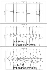
Wedge modelling is often used to understand the vertical (thin bed) resolution limits of seismic. The wedge model is a high AI layer embedded in a low AI surrounding. As used in Figure 3, it consists of 11 traces, and thickens from 1 ms on the left to 51 ms on the right. Each trace (not shown) contains two reflectivity spikes of equal amplitude but opposite sign. The top spike is located at the top of the wedge. The bottom spike is located at the bottom of the wedge. To investigate the effect of low frequencies in the wavelet, we filter the model traces with impedance wavelets of 2.5–50 Hz and 10–50 Hz. Note the side-lobe reduction and improved interpretability of the wedge when low frequencies are filled in. This example is a key result showing the benefit of low frequencies as it nicely illustrates the value for seismic interpretation.
Spatial resolution
Equally as important as temporal resolution is the issue of spatial resolution. The most common way to discuss spatial resolution is in the context of Fresnel zones. However, that discussion typically deals with resolution before seismic migration – the noble mathematical art of transforming seismic data into a ‘true’ image of the subsurface. We are interested in resolution after migration. To this end, we follow the method proposed by Berkhout (1984) for quantifying spatial resolution, via the use of the post-migration ‘spatial wavelet’. The spatial wavelet is simply the migrated point diffractor’s response after bandlimiting the temporal spectrum.
The two key parameters dictating the nature of the spatial wavelet are the temporal bandwidth and the spatial aperture. Figure 4 (top) shows three spatial wavelets for a single point diffractor in a constant-velocity medium. The temporal bandwidths are varied in the same way as in Figure 1, i.e. the maximum frequency value is varied while holding the minimum frequency fixed. As expected, the larger FMAX values yield sharper spatial wavelets. Thus, better temporal resolution also leads to better spatial resolution.
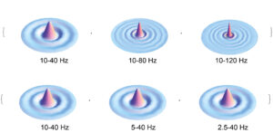
Figure 4 shows three more spatial wavelets for the same medium. This time the FMIN value is changed while holding FMAX fixed. Again, the trends are the same as in the temporal case. In other words, the main lobe shows hardly any change while the side lobes diminish as FMIN is lowered. The side lobes are difficult to see in the figure, but a closer look would reveal that the side lobes diminish with lower FMIN.
References:
A. J. Berkhout, 1984. Seismic Resolution: a Quantitative Analysis of Resolving Power of Acoustical Echo Techniques. Geophysical Press, London
M. S. Egan, 2005. The drive for better bandwidth and resolution: Petroleum Geology Conference series 6 1415-1424
R. S. Kallweit and L. C. Wood, 1982. The limits of resolution of zero-phase wavelets: Geophysics 47 1035–1046
Follow link for Part II