Know Your Faults! Part I
In Part I of this series, we look at the geometric representation and identification of faults. In the final part, we review slip classification, stress orientations and tectonic styles of faults.
In 1921, Richard Oldham delivered his presidential address at the annual meeting of the Geological Society of London; taking inspiration from an ancient maxim that ‘to know your faults is the greatest wisdom’, Oldham entitled his talk, ‘Know Your Faults’. Decades later, detailed mapping and improved visualisation techniques have revealed even more the association of faults of various types and sizes with petroleum basins. Faults play key roles in the genesis and evolution of sedimentary basins and petroleum traps and in the migration of fluids and compartmentalisation of reservoirs. That all these processes are associated with faults indicates their complex, varied nature and necessitates a proper understanding of faults in basin tectonics, subsurface mapping, seismic interpretation, petroleum system modelling, and reservoir simulation.
Faults are a core subject in structural geology and may be studied from three different perspectives: (1) the geometry and architecture of faults, (2) the stresses that form faults (geomechanics), and (3) the sequential, temporal development of faults in a given area (kinematics). All these aspects are inter-related and need to be incorporated in a comprehensive study; fault geometry is the end-member of kinematics, which is, in turn, caused by stresses. Here we look at some key terms and concepts that describe the geometry of faults.
Fault Definitions
The concept of faults entered geology in the late 18th century via observations made by coal miners in mountain excavations. In his celebrated Principles of Geology (volume 4, 1835) Sir Charles Lyell wrote: “A Fault, in the language of Miners, is the sudden interruption in the continuity of strata in the same plane, accompanied by a crack or fissure varying in width from a mere line to several feet, which is generally filled with broken stone, clay, etc.”
 Stratigraphic identification of normal and reverse faults in wells. Note also that unit 3 is syntectonic sediment thickening in the down-going fault block. Source: Rasoul Sorkhabi (2012)
Using this statement as a portal of entry into our discussion, two points are noteworthy. First, faults are fractures or rupture planes along which the opposite walls of a rock column have moved relative to each other. The rock block above the inclined fault plane is called the hanging-wall because miners could hang their lamps on that block; the block below the fault plane is called the footwall where the miner placed his feet. The second point is that a fault is not a smooth plane (as textbooks show for simplicity) but a concentrated zone of deformation. A fault zone often consists of crushed, brecciated or highly sheared fault rock surrounded by a damage zone characterised by fractures, hydrothermal veins, etc. Faults with greater lengths also have thicker fault zones. The nature of the fault zone depends firstly on the type of host rock; hard sandstones may show intense fracturing along the fault while ductile mudstone may smear into fault plane. Secondly, the nature of the fault zone depends on crustal depth. At deeper levels, where temperatures of over 300°C and higher pressures are prevalent, fault zones will undergo ductile deformation (as in metamorphic terrains); while in the upper eight kilometres of the crust, which also includes the majority of sedimentary basins, fault zones will show brittle deformation.
In Search of Faults
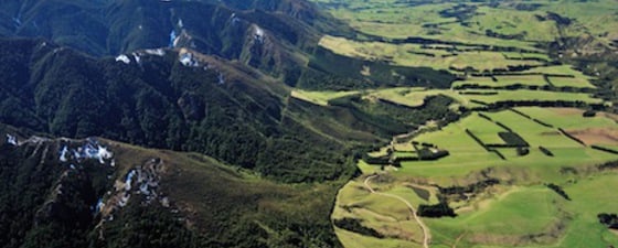
 Geometric relations in a faultTectonic faults are generated at crustal depths. A blind fault is one that still lies beneath the Earth’s erosional surface (although it may have a topographic expression). An emergent fault is marked by a fault line (or fault trace) and may produce a steep topographic surface called a fault scarp.
Depending on the type of available data, there are several indicators to identify fault structures. These include: (1) topographical features such as lineaments, offset streams, fault scarps, etc.; (2) discontinuity in a marker bed in an outcrop section; (3) juxtaposition of rocks of different ages (reverse faults often bring older rocks atop younger rocks while normal faults have younger rocks at their hanging-wall contacts); (4) features associated with fault zones such as gouge (‘fault flour’), slickenside (smooth, striated fault surface), intense fracturing, sheared rock fabric, hydrothermal veins, etc.; (5) geophysical indicators such as displaced seismic reflectors or gravity anomalies in a particular pattern; (6) repetition (by reverse faults), omission (by normal faults) or downthrown-side thickening (by growth faults) of strata in borehole records (cores and logs). Ideally, several indicators should be used to better characterise a fault system.
Whether a fault is active or not has enormous relevance not only for construction of dams, bridges and other structures but also for oil and gas fields. An active fault is usually defined as one for which there is earthquake evidence in the past 10,000 years (the Holocene) while inactive faults have not moved for the past 1.6 million years (the Quaternary). Nevertheless, any fault is a plane of weakness and is prone to reactivation if sufficient stress is applied.
Faults come in various sizes. Fault structures are on the scale of at least metres, minor faults or sheared fractures on the scale of centimetres, and microfaults (or microfractures) on the scale of millimetres. On seismic images, faults are prominent features as they displace and distort the reflectors from sedimentary layers. However, even with the best seismic images, the population of smaller faults (say with offsets of less than 5 or 10m depending on seismic quality), which are below the seismic resolution, are not visible; these are called sub-seismic faults.
In the early 20th century, the American geologist Raphael Pumpelly suggested that in a given area small faults mimic the shape and orientation of larger structures of the same generation. In 1970, J. S. Tchalenko published an influential paper in the GSA Bulletin showing how tectonic stresses can give rise to self-similar shear structures at various scales. With the rise of the fractal theory of natural phenomena, geologists have tried to model populations of faults as a scale-invariant fractal distribution. While this is theoretically a powerful tool, for instance to predict the population of sub-seismic faults in a basin, its application is far from perfect and requires better calibrations from massive empirical data and detailed understanding of fault development.
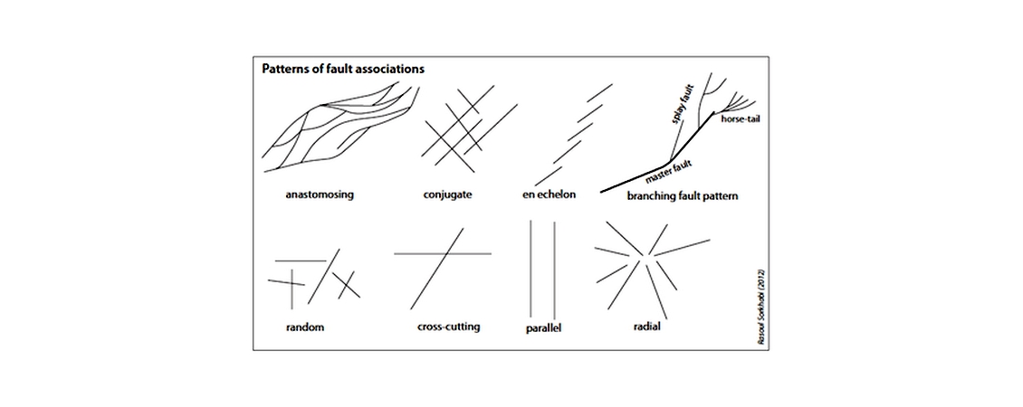
Fault patterns. (Source Rasoul Sorkhabi)
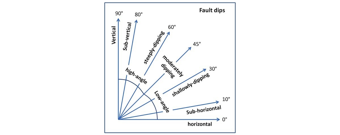
Fault Dips. (Source Rasoul Sorkhabi)
Geometric Representation
 This outcrop photo shows a normal fault in the Bozeman Group (continental Tertiary sediments) near the Harrison Reservoir, Montana, USA. Source: Dr. Michael C. Rygel of State University of New York, College at Potsdam.A fault is geometrically characterised by its strike, dip, displacement, throw (vertical offset), heave (horizontal offset), and sense of movement. Faults with dip angles of over 45° are high-angle, while those dipping less than 45° (or less than 30° according to some geologists) are low-angle faults. The amount of fault displacement typically depends on fault length: a 100 km long fault may have a displacement of 1 km. Quantifying the relationship between these two parameters is the subject of many recent studies because by knowing one parameter we may predict the other; however, empirical data also show complexities resulting from lithology, fault type, and methods of analysis.
Depending on the type of data acquisition, faults are depicted in various ways: surface (2D planar), maps views (geologic maps on topographic sheets and lineament maps on satellite images), cross-sections (profiles), 3D block diagrams, subsurface structural counter maps, 2D or 3D seismic images, and fault surface maps with juxtaposed strata, curvature, and so forth.